Resistor Grids and Matrix Square Roots

In two previous notes we discussed the resistances between the nodes of an infinite square lattice of resistors. In the first we derived an analytical expression for those resistances, using the standard naïve approach, and in the second we derived a matrix expression for the resistances. In both we made use of superposition arguments, developing the field of voltages for opposite “monopoles”, and then superimposing them to give a closed current path. However, we also noted that the absolute values of the voltages in those monopole solutions don’t converge; only the differences between voltages converge. To derive the exact analytical expressions for the voltages by this method, we would like to re-express it in terms that explicitly give zero voltage at the origin. In the following, we’ll show explicitly why the expression developed in the previous note leads to infinite voltage at the origin, and we’ll develop a more general solution that can be expressed in “closed form”, and that can be tailored to give zero voltage at the origin. We’ll find that that the solution of this infinite grid of resistors essentially reduces to simply evaluating the square root of a matrix. Several similarities between this problem and the mathematical aspects of quantum mechanics and quantum field theory are noted.

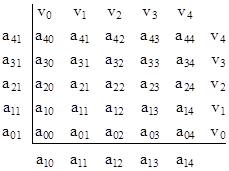
First, consider the voltages in one quadrant of the finite square lattice, as shown below.

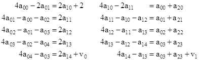
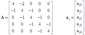
In addition to the symmetry of the four quadrants, the values in each quadrant are symmetrical about the main diagonal, i.e., we have a_ij = a_ji. The symbols v_j denote boundary conditions. With unit resistors between each pair of adjacent nodes, the equations governing this system are

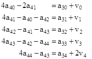
and so on. The last set of equations (for the values adjacent to the upper boundary) is

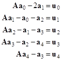
In matrix form these sets of equations can be written as

where

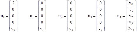
and

If all the boundary values v_j are set to zero, this system of equations is identical to the one developed in the previous note. Hence the previous derivation tacitly imposed zero voltage at the boundary, which then requires the voltage at the origin to approach infinity. To find a solution with zero at the origin, the boundary values must approach infinity. Although we’ve distinguished five values v₀ to v₄ along the boundary, we saw in a previous note that in order to yield the desired “realistic” solution we must set these boundary values equal to each other. Therefore, we will set each of the values v₀ to v₄ equal to the a single value denoted by v.

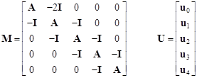
Just as in the previous note, we can write the system of matrix equations in the form of a meta-matrix equation as follows

where

We can solve this system symbolically as a = M^–1U to give the voltage at each node of the lattice. Only a₀ is actually needed, since the other vectors follow easily once a₀ is determined. The discussion so far has focused on a finite lattice of size N = 4, but the same formal system of equations arises for any N. With N = 7 we get

With all the v_j values equal to a single value v, this expression can  be written in simplified form as

where

Again we see that if v = 0 the solution reduces to that given in the previous note, corresponding to the condition of zero voltage at the boundary. In that case we had simply

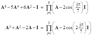
and by making use of the known roots of the polynomials in A, we found that for any odd N this could be expressed as

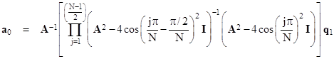
To simplify this further, notice that by applying a suitable phase shift to the arguments of the sine function, we can re-write this purely in terms of cosine functions as

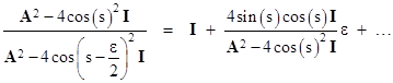
For sufficiently large N, the quantities s(j) = jπ/N for j = 1 to (N–1)/2 vary almost continuously from 0 to π/2, the offset ε = π/N becomes infinitesimally small, and the step size for the s values is ε, the range limits of the product approach s = 0 to (π/2)/ε. We can expand the argument of the product in powers of ε as

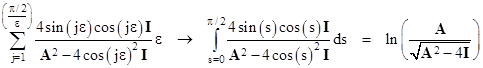
Taking the natural log of the product, and noting that ln(1+kε) approaches kε, we can convert the product to a summation and then to an integral in the limit as N increases to infinity

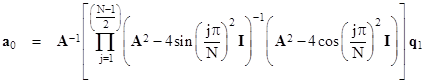
Taking the exponential and inserting this for the product back into the expression for a₀, we get, in the limit as N increases to infinity, the result

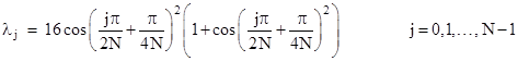
Although this is more succinct than the explicit product form, it is equivalent – in the limit of increasing N – to the product form, with the same numerical difficulties as we increase the dimensions of A, because the voltage at the origin diverges to infinity. Still, it’s of interest to see how this expression is evaluated. To take the square root of the matrix in the denominator we make use of the trigonometric eigenvalues of the matrix W = A² – 4I. For any even value of N (the dimension of the A matrix), the eigenvalues of W are

In terms of the matrices G and Z defined by

where C = [1 1 1 … 1]^T, the similarity transformation matrix P that diagonalizes W is given by

Note that the columns of P are simply the eigenvectors of W. Letting H denote the inverse square root of the diagonalized matrix P^–1WP, we have

Applying the inverse transformation and inserting into the expression for a₀, we get

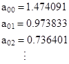
In principle this can be used to compute the components of a₀ for any N. It gives reasonably good approximate values for relatively small N. For example, with N = 16 it gives

Thus the resistance from the origin to the next adjacent vertex is 0.500257…, and to the next vertex is 0.72779… , compared with the exact analytical values of 0.5 and 0.72676… respectively. However, as N increases, it becomes necessary to carry out the computations with more and more significant digits to avoid losing accuracy. As discussed previously, the value a₀₀ at the origin goes to infinity, because with v = 0 we are forcing the boundary voltages to be zero.

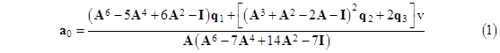
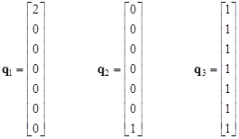
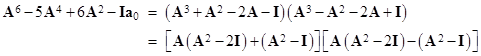
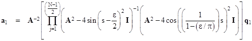
Returning to the more general expression (1), with v not equal to zero, notice that the coefficient of q₂ is simply the square of the polynomial in A that has the “even” ordered trigonometric roots of the polynomial that is the coefficient of q₁. For example, the coefficient polynomials in equation (1) are related by

Thus the linear factorizations of the coefficient polynomials are

Using this we could develop a closed-form expression for all the terms of (1), but this turns out to be unnecessary, because the coefficient of v in equation (1) reduces to the identity column C = [1 1 1 … 1]^T. For example, with N = 7 we have

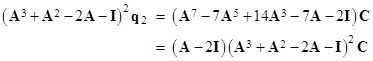
Noting that q₃ = C, this can be written as

Bring the 2C over to the right side, and factoring, we get

Multiplying through by the inverse of the left hand factor, this can be written as

Moreover, the similarity transformation on the right side yields A – 2I, so we have

which signifies that these two matrices commute. The preceding relation then merely expresses the fact that each row of A – 2I sums to zero except for the last, which sums to 1.

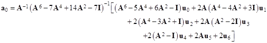
From the above discussion it follows that, for any given boundary voltage v, equation (1) simplifies to

To make a₀₀ equal to zero we must set v equal to the magnitude that a₀₀ would have with zero voltage at the boundary. Unfortunately this value approach infinity as the size of the grid increases. A slightly different approach to producing a finite limiting vector is to allow v to be zero but compute the difference a₀ – a₁. We saw in a previous note that a₁ (for the case N = 7) is given by

Making use again of the trigonometric form of these polynomials, this can be written as

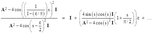
Notice that the factors of A^–1 and A in the previous expression cancel, but we apply a new factor of A^–2 to the entire product to cancel the extra factor in the numerator when j = 3. As in the case of our evaluation of a₀, we define ε = π/N, and we convert the sines to cosines by shifting the arguments by –ε/2. However, in this case the argument of the cosine in the numerator must be adjusted because it is divided by N–1 instead of N, so the argument is sN/(N–1) instead of simply s. Thus we write

As before we expand each argument of the product in powers of ε, and we get

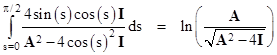
Taking the natural log of the product, we can convert the product to a summation. Noting that our variable s = jπ/N ranges from 0 to (π/2)/ε, and taking the limit as ε goes to zero (and N goes to infinity), we get an integral of two terms, the first being identical to the one we encountered when evaluating a₀, namely,

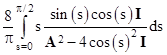
To this we must add the integral of the second term

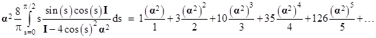
This integral is a bit more challenging, but we can evaluate it by some manipulation of series expansions. Letting α = A^–1, we can expand the integral into a power series in α as follows

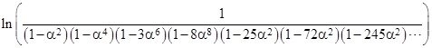
The numerators of the coefficients 1, 3, 10, 35, 126, … are the central binomial coefficients for odd orders. This same series is also given by

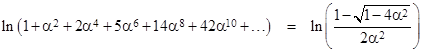
The product inside the logarithm involves the series 1, 1, 3, 8, 25, 72, 245, … , whose values might not seem easily expressible in closed form, but if we expand this argument in a series we find that it’s coefficients are the Catalan numbers, 1, 1, 2, 5, 14, 42, …, so the expression can be replaced with the known generating function, i.e., the above logarithm equals

Combining these results and inserting back into the expression for α₁, we get (in the limit as N approaches infinity)

As with a₀, the components of this vector approach infinity, so it’s difficult to draw conclusions about the limit as N increases. Perhaps a more useful approach is to evaluate the difference between a₀ and a₁, since this difference converges on a finite vector of values. From these differences we can easily compute all the resistance values, and indicated in the figure below.

Knowing the difference between a₀₀ and a₁₀, we know by symmetry the value of a₁₀, and then since we know the difference between a₀₁ and a₁₁ we know a₁₁. Then, given these values, the value of a₀₂ is given by the relation 4a₀₁ = a₀₀ + 2a₁₁ + a₀₂. We also know the difference between a₀₂ and a₁₂, so we know a₁₂, which enables us to compute a₀₃, and so on. Likewise all the other voltages in the grid can easily be computed.

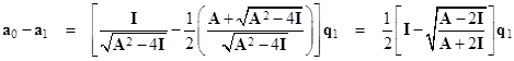
To determine the difference between a₀ and a₁, we combine equations (2) and (4) to give the relation

Letting I – Ψ denote the matrix inside the square root, and noting that q₁ is a column vector with 2 as the uppermost element and zero for the remaining elements, we see that a₀ – a₁ is simply the first column of

By definition the matrix Ψ satisfies the relation

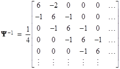
so the inverse is

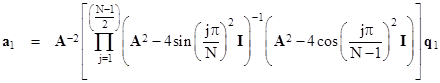
For any N x N matrix of this form the eigenvalues are

In terms of the matrices G and Z defined by

where C = [1 1 1 … 1]^T, the similarity transformation matrix P that diagonalizes Ψ^–1 is given by

Again we note that the columns of P are simply the eigenvectors of Ψ^–1. Letting D denote the diagonal matrix given by P^–1(Ψ^–1)P, we have (Ψ^–1) = P(Dⁿ)P^–1. Making this substitution, we can write the series expression (5) as

Letting H denote the diagonal matrix in the square brackets, we have

It follows that a₀ – a₁ is the first column of

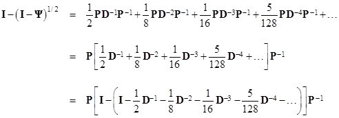
where χ = [1 0 0 … 0]^T. Thus the solution of the infinite grid of resistors consists essentially of just taking the square root of a matrix. Of course, another way of evaluating the square root of I – Ψ would be to take the exponential of half the logarithm, but this again leads to a sum of powers of Ψ.

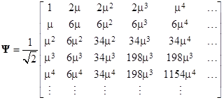
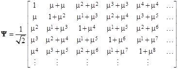
Incidentally, if we try to evaluate (5) directly in terms of Ψ rather than its inverse, we find that in the limit as N increases, the Ψ matrix converges on

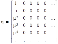
where

and the coefficients 2, 6, 34, 198, 1154, … etc., satisfy the recurrence s_n = 6s_n–1 – s_n–2. From this it follows that the nth coefficient is given by s_n =  μⁿ + μ^–n, so the Ψ matrix can be written explicitly as

It’s interesting that μ also figures prominently in the analytic solution described in a previous note. Letting s and c be the matrices with components

we can write

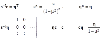
where

Some interesting relationships involving these matrices are

Many similarities exist between the infinite resistor grid problem, quantum mechanics, and quantum field theory. For example, we often deal with infinite matrices in quantum mechanics, and in quantum field theory we encounter logarithmic divergences in some of the quantities, leading us to establish various cutoff schemes. Likewise in Feynman’s approach to quantum field theory the Dirac delta function is initially introduced, but then replaced with a slightly less “sharp” function, and it is found that the ultimate answers are insensitive to the sharpness. We’ve seen above that the infinite grid of resistors can be modeled by a matrix that is nearly the delta matrix, i.e., it has the constant along the main diagonal, and most of the off-diagonal terms are zero, but the terms immediately adjacent to the diagonal are non-zero. We take this matrix to the limit of infinite dimensions, so it is nearly a purely diagonal matrix. It’s also interesting that when the solution of the resistor grid problem is expressed as a integral and we attempt to evaluate the integral numerically, it tends to be poorly behaved unless we impose some cutoff limit on the bounds of integration – which is similar to the situation in quantum field theory. Also, we note that the taking of the square root of an infinite matrix figures prominently in quantum field theory, just as it does in the infinite resistor grid problem. Lastly, the lack of uniqueness of the “vacuum” solutions, and the dependence on the polarization of the vacuum is important both in quantum field theory and in the infinite resistor grid problem.

Return to MathPages Main Menu