|
The Algebra of an Infinite Grid of Resistors |
|
|
|
In a previous note we discussed the well-known problem of determining the resistance between two nodes of an “infinite” square lattice of resistors. The most common approach is to superimpose two “monopole” solutions, one representing the field for one amp of current entering a given node and flowing “to infinity”, and the other representing the field for one amp of current being withdrawn from a given node flowing in from infinity. If the two nodes are adjacent, the solution is fairly unambiguous, but the resistance between two arbitrary nodes of an “infinite” resistor grid is actually indeterminate unless we impose restrictions on the voltage and current levels “at infinity” (such as stipulating that we seek the solution for a finite grid in the limit as the size of the grid increases to infinity). |
|
|
|
According to the naïve approach, we imagine injecting 1 amp of current into a single node at the origin, and allow it to flow outward symmetrically to infinity. Let Vm,n denote the voltage drop from the source node with coordinates (0,0) to any given node with coordinates (m,n). Likewise we could imagine extracting one amp from the node at (m,n), flowing in symmetrically from infinity, and the voltage drop from the origin to (m,n) would also be Vm,n. Superimposing these two solutions, we have one amp entering node (0,0) and exiting node (m,n), and the voltage drop is 2Vm,n, so the net effective resistance between (0,0) and (m,n) is Rm,n = 2Vm,n/I, where I = 1 amp. Of course, as mentioned in the previous note, the voltage “at infinity” must go to infinity relative to the voltage at the source, because the resistance to infinity is infinite. Nevertheless, it might seem that with suitable care we can evaluate the limit to arrive at an unambiguous answer. |
|
|
|
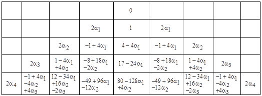
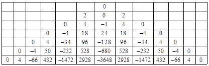
However, the stated problem has a unique solution only if we stipulate some restriction on the boundary conditions. This is a delicate proposition, since the boundary is “at infinity” and the voltage approaches infinity. The ambiguity can be seen immediately by examining the figure below, which shows a node from which two amp of current is being extracted, surrounded by nodes of higher voltage necessary to supply this current. The figure shows just the lower quadrant of the grid, with the understanding that that other three quadrants are symmetrical. The voltages along the diagonals are denoted by α1, α2, α3, …, and all the other voltages are expressed in terms of these, in such a way that the difference equation governing the system is satisfied. |
|
|
|
|
|
|
|
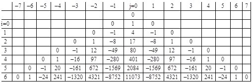
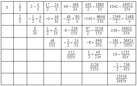
For a grid with 1 ohm resistors between each pair of adjacent nodes, the effective resistance between the origin and any given node equals half the value listed for the node in the table below. Obviously this construction can be continued to infinity, since each succeeding row is computable from the prior rows, noting that the outer-most cells adjacent to the diagonals are determined by symmetry with the neighboring quadrants. Thus for any arbitrary choice of the diagonal parameters α1, α2, α3, …, we can construct an entire infinite grid. For example, if we set all the diagonals to zero, we get |
|
|
|
|
|
|
|
We will refer to the value in the ith row and jth column of this array as ρi,j. The sum of the terms of the nth row is n. The terms are generated by the basic two dimensional recurrence (representing the discrete form of the Laplace equation) |
|
|
|
|
|
|
|
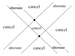
This table implies that the resistance between the origin and any node on either diagonal is zero. Does this mean that an infinite grid of resistors acts as a superconductor with zero resistance between two arbitrarily distant nodes? (It’s interesting to compare this with the pseudo-metric of Minkowski spacetime, in which the “diagonals” represent light-like intervals of null magnitude.) Notice that we achieved this “superconductivity” along the diagonals at the expense of introducing large voltages and currents at the off-diagonal nodes. The fact that these voltages increase to infinity is not really objectionable, because any monopole solution must have the voltages increasing to infinity as we move away from the origin. On the other hand, we might object to the fact that the voltages alternate between positive and negative values on adjacent nodes in the transverse direction, and hence the transverse currents between adjacent nodes go to infinity. However, nothing in the original problem statement restricts the behavior of the voltages and currents at arbitrarily large distances from the origin. The only requirement is to specify a set of voltages and currents on the infinite grid that everywhere satisfy Ohm’s Law across each resistor, with a certain amount of current entering one particular node and exiting one other particular node. One might argue that the superposition of the two monopole solutions yields finite behavior at infinite distances from the two monopoles, because the infinities of the individual monopole solutions cancel each other, but it’s conceivable that similar cancellation could occur for superpositions of diagonally null grids. Notice that the signs alternate by columns in the “past” and “future” regions, and by rows in the “present” regions, so if the two poles are separated by an even number of nodes in both directions, they will tend to cancel (i.e., destructively interfere with each other) in all regions except along the stripes between their null diagonals, as shown below. |
|
|
|
|
|
|
|
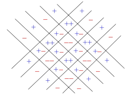
In the “light-like” regions between the two interacting poles, the voltages and currents are alternately re-enforcing and canceling, as depicted below. |
|
|
|
|
|
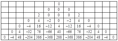
This could be regarded as an analog to polarized vacuum solutions of the Laplace equation. Of course, rather than setting the diagonal voltages to zero, we can set them to any values we choose. The result is given by superimposing the “null” solution (whose values were given in the preceding table) with the product of each diagonal value times the corresponding array that satisfies the usual Laplace recurrence relation (noting that the recurrence for the nodes adjacent to the diagonal actually involve the symmetrical nodes in the neighboring quadrant). For example, if α1 is not zero, we must superimpose α1 times the array shown below. |
|
|
|
|
|
|
|
Similarly, if α2 is not zero, we must superimpose α2 times the array shown below. |
|
|
|
|
|
|
|
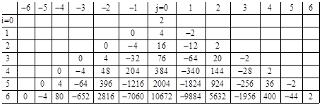
And so on. In general, each of these arrays consists of the superposition of two mirror-symmetrical arrays, with their vertices placed at the locations of the respective αj, and having the values shown in the table below for the left hand side, and reflected for the right hand side. For future reference, we refer to the value in the ith row and jth column of this array as σi,j. |
|
|
|
|
|
|
|
By selecting suitable values of α1, α2, α3, … we can make the effective resistance between any two (non-adjacent) nodes anything we like. Whether such solutions are physically meaningful is questionable – but no more so than the physical meaningfulness of an “infinite” grid of resistors. No such physical entity can exist, so we have no basis for claiming that we know how it would behave. (Even if we accepted the existence of an actual infinite grid, it would necessarily have capacitance and inductance so that the propagation speed was finite, and hence no equilibrium state could come into existence in finite time.) We can certainly examine the behavior of finite grids of progressively larger sizes, and note that the steady-state behavior near the center of such grids approaches a unique limit, but we are not justified in claiming that this limiting behavior for large finite grids is even qualitatively the same as the behavior of a (hypothetical) truly infinite grid. (In calculus, the fallacy that the limit of a sequence must possess the limiting attributes of the members of that sequence underlies what is known as the Limit Paradox.) Before dismissing such considerations as purely academic, it’s well to remember that the fundamental relation pq – qp = –ihI for position and momentum matrices in quantum mechanics relies on the existence of infinite matrices with terms that increase to infinity. The relation is algebraically impossible for any finite or “well-behaved” matrices (as can be seen by considering the traces of the products). |
|
|
|
Incidentally, there are stories about job applicants being asked questions about the hypothetical “infinite grid of resistors” during job interviews, by certain organizations that ostensibly value abstract problem solving talent. Ironically, the reasoning behind the standard solution is sufficiently questionable that one could argue that the applicants who declare they can’t solve the problem are actually more insightful than the ones who give the standard solution. At the very least, the question should either be posed in terms of the limit of increasingly large but finite grids, or else some constraint on the behavior “at infinity” must be specified. Otherwise, the answer is completely indeterminate. (The standard answer for adjacent nodes is arguably less ambiguous than for other pairs of nodes, but even in that case the superposition method involves the concept of flowing current into a grid of infinite resistance.) |
|
|
|
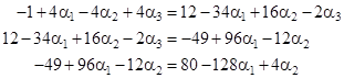
Recognizing that some “physically reasonable” constraint must be placed on the behavior at infinity in order to determine a unique answer, we might ask what constraint is sufficient. In the table showing the complete solution in terms of the arbitrary diagonal parameters, suppose we stipulate that, for some n, the voltages along the outer perimeter of the nth concentric square (excluding the corners for n > 1) are all equal to each other. If we impose this on the first concentric square, we have the condition 2α1 = 1, from which we get α1 = 1/2, but of course this leaves the rest of the diagonal voltages indeterminate. If we impose the condition on the perimeter of the second concentric square, we have -1 + 4α1 = 4 – 4α1, which implies α1 = 5/8 = 0.625. If, instead, we impose the condition on the third concentric square, we get two equations |
|
|
|
|
|
|
|
Solving these two equations in two unknowns, we get |
|
|
|
|
|
|
|
Applying the condition to the 4th concentric square, by equating the expressions for adjacent nodes on the perimeter of that square, we get the following three conditions |
|
|
|
|
|
|
|
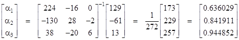
Solving this linear system of three equations in three unknowns, we have |
|
|
|
|
|
|
|
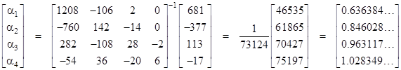
If we impose the uniformity condition on the perimeter of the 5th concentric square, and solve the resulting system of four equations in four unknowns, we get |
|
|
|
|
|
|
|
Clearly if we impose the uniformity condition on the perimeter of the (n+1)th concentric square we get a linear system of n equations that can be solved for the first n diagonal parameters, and these parameters converge on specific values as n increases. From these diagonal terms, all the remaining terms are easily computed, as shown above. Thus we have a straightforward algebraic way of solving, in principle, for the resistance between any two nodes – at least numerically – for a finite square grid with uniform boundary. In general the vector α of voltages α1, α2, …, αN-1 along the diagonal for any given N (i.e., imposing uniformity on the (N+1)th concentric square) are given by |
|
|
|
|
|
|
|
where the components of S and V are expressible in terms of the previously defined “ρ” and “σ” arrays as |
|
|
|
|
|
|
|
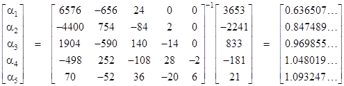
For example, with N = 5 (i.e., imposing uniformity on the 6th concentric square) we get |
|
|
|
|
|
|
|
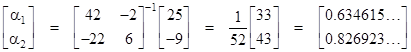
For one more example, with N = 6 we get |
|
|
|
|
|
|
|
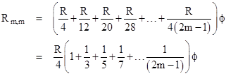
By this method we can approach arbitrarily close to the limiting values as the grid side increases. However, this doesn’t provide an exact analytical expression for the limiting values. We would like to determine whether there are simple closed-form expressions for these resistances. One approach is to notice that the central node is connected to the first concentric square by 4 links in parallel, and this square is connected to the next by 12 links in parallel, and this square is connected to the next by 20 links in parallel, and so on. Therefore, we expect the resistances from the origin to the corners of the mth concentric square to be roughly |
|
|
|
|
|
|
|
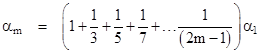
for some constant ϕ. In other words, we conjecture that the voltages at the corners of the concentric squares are proportional to the partial sums of the odd geometric series, which is to say |
|
|
|
|
|
|
|
For example, we expect α2 to approach (1 + 1/3) = 1.3333… times α1 as the grid size increases, and we find support for this in the preceding algebraic solution for N = 6, which gave α2/α1 = 1.3323… Likewise α3/α1 seems to be approaching (1 + 1/3 + 1/5), and so on. Of course, we already know that the choice of the diagonal parameters is arbitrary, so we are free to impose this constraint on the values of those parameters. The question is merely whether, for some value of α1, the resulting behavior “at infinity” for the entire grid satisfies whatever constraints we choose to impose. |
|
|
|
As noted above, the requirement for uniform voltage along the perimeter of the 4th concentric square implies, for the two nodes closest to the corner, the equality |
|
|
|
|
|
|
|
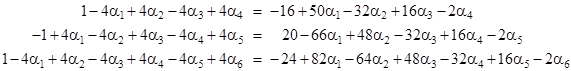
The corresponding conditions for the next few concentric squares are |
|
|
|
|
|
|
|
As we proceed to larger and larger squares, the left hand contributions to the coefficients of the α parameters do not increase, but the right-hand contributions increase linearly. Specifically, the magnitudes of the coefficients on the right side are 4n, 16(n-1)+2, 16(n-2), 16(n-3), …, 16(1), 2. In the limit as n increases, only the factors proportional to n affect the final result, so the limiting condition is |
|
|
|
|
|
|
|
Letting sn denote the nth partial sum of the odd harmonic series, i.e., |
|
|
|
|
|
|
|
our conjecture is that αn = snα1, and hence the prior equation can be written as |
|
|
|
|
|
|
|
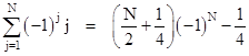
Making use of the identity |
|
|
|
|
|
|
|
and noting that as N increases to infinity the right hand side is proportional to ±N/2, the preceding equation for sufficiently large n approaches |
|
|
|
|
|
|
|
Therefore, in the limit as n increases to infinity, we have |
|
|
|
|
|
|
|
The infinite series in the square brackets, sometimes called Leibniz’s series, is easily shown to equal p/4, so it follows that |
|
|
|
|
|
|
|
By the same analysis we can show that, equating the voltages of each pair of adjacent nodes on the perimeter leads to the same conclusion. For example, the coefficients of the voltage for the next node are of the form 32(n-j)2 – 24(n-j) + 396, and equating the voltage of this node to that of the previous node leads to the asymptotic equation |
|
|
|
|
|
|
|
Noting that the sum of the squares up to N2 with alternating signs is asymptotic to N2/2, this again leads to the conclusion that α1 = 2/π. One might argue that, instead of evaluating the right side of the above equation and then dividing through by n2 and showing that the coefficients of 1, 1/3, 1/5, etc, approach ±1, we could just as well have divided through the above equation by n2 immediately, which seems to imply that the coefficients of s1, s2, s3, etc., approach ±1. On this basis, the partial sums alternate between 1 + 1/5 + 1/9 + 1/13 + … and -1/3 – 1/7 – 1/11 – 1/15 - … However, the asymptotic average of these two sums if π/8, which again leads to α1 = 2/π. But working out the sums exactly for any finite case shows that the partial sums are actually all positive, and they converge uniformly, consistent with evaluating the right hand side of the above equation prior to dividing through by n2 and taking the limit. |
|
|
|
From this, the voltages (and hence the resistances) from the origin to every other node of the grid can easily be given in closed form. The table below gives the resistances (in ohms) between the origin and each of the surrounding nodes, assuming each lattice resistor is 1 ohm. |
|
|
|
|
|
|
|
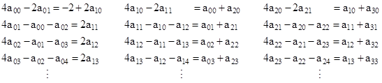
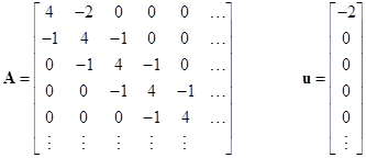
Another approach is to simply arrange the system equations into a meta-matrix of matrices for a monopole solution, similar to the approach taken in a previous note on the dipole solution. Letting amn denote the voltage at node (m,n), the system equations are |
|
|
|
|
|
|
|
and so on. If we define the column vectors aj = [aj0, aj1, aj2, …]T, these equations can be written in the form |
|
|
|
|
|
|
|
where |
|
|
|
|
|
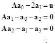
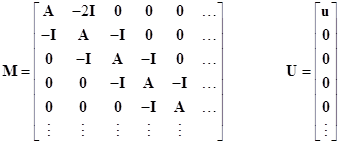
These matrix equations can then be written as a meta-matrix equation, whose coefficient matrix is formally identical to the coefficient matrix of the individual matrix equations. Thus, letting a denote the meta column vector a = [a0, a1, a2, …]T, and letting I denote the identity matrix, the overall system equation can be written as |
|
|
|
|
|
|
|
where |
|
|
|
|
|
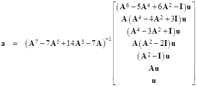
The formal similarity of the meta matrix M and the matrix A is to be expected, since these two levels represent the evaluations of the rows and columns, and they could just as well be reversed, treating the columns at the first level and the rows at the meta level. The solution, giving the voltages at every node, is simply a = M–1U. To evaluate this, first consider a finite example, truncated at just seven rows and columns. Formally this gives |
|
|
|
|
|
|
|
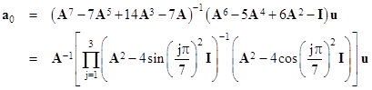
The elements of this expression are Legendre polynomials, whose roots are just 4 times the squares of the sines or the cosines of fractional multiples of π. This enables us to write the general solution in a simple product form. For example, the vector a0 is given as |
|
|
|
|
|
|
|
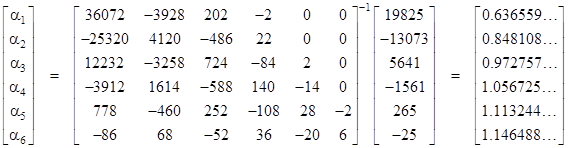
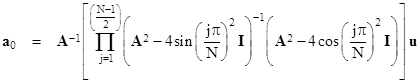
In general, for any odd N, with the A, u, and I matrices defined to order N, we have |
|
|
|
|
|
|
|
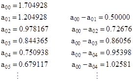
This already gives good results for relatively small values of N, and the accuracy improves as N increases. For example, with N = 39 we get |
|
|
|
|
|
|
|
These drops in voltage agree with the closed form analytical expressions derived previously. Note that the values of a0 are sufficient to determine all other values by simple recursive application of the Laplace equation. The drawback of this approach is that the absolute values of the voltages don’t converge; only the differences between voltages converge. To derive the exact analytical expressions for the voltages by this method, it would probably be necessary to re-express it in terms that explicitly give 0 voltage at the origin. This is discussed further in another note. |
|
|