Infinite Grid of Resistors

                  Remain, remain thou here,

While sense can keep it on. And, sweetest, fairest,

As I my poor self did exchange for you,

To your so infinite loss, so in our trifles

I still win of you: for my sake wear this...

                                                          Shakespeare

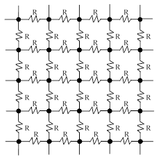
There is a well-known puzzle based on the premise of an “infinite” grid of resistors connecting adjacent nodes of a square lattice. A small portion of such a grid is illustrated below.

Between every pair of adjacent nodes is a resistance R, and we’re told that this grid of resistors extends “to infinity” in all direction, and we’re asked to determine the effective resistance between two adjacent nodes, or, more generally, between any two specified nodes of the lattice.

For adjacent nodes, the usual solution of this puzzle is to consider the current flow field as the sum of two components, one being the flow field of a grid with current injected into a single node, and the other being the flow field of a grid with current extracted from a single (adjacent) node. The symmetry of the two individual cases then enables us to infer the flow rates through the immediately adjacent resistors, and hence we can conclude (as explained in more detail below) that the effective resistance between two adjacent nodes is R/2. This solution has a certain intuitive plausibility, since it’s similar to how the potential field of an electric dipole can be expressed as the sum of the fields of a positive and a negative charge, each of which is spherically symmetrical about its respective charge. Just as the electric potential satisfies the Laplace equation, the voltages of the grid nodes satisfy the discrete from of the Laplace equation, which is to say, the voltage at each node is the average of the voltages of the four surrounding nodes. It’s also easy to see that solutions are additive, in the sense that the sum of any two solutions for given boundary conditions is a solution for the sum of the boundary conditions.

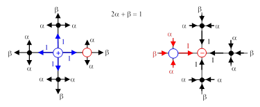
If we accept the premise of an infinite grid of resistors, along with some tacit assumption about the behavior of the voltages and currents “at infinity”, and if we accept the idea that we can treat the current fields for the positive and negative nodes separately, and that applying a voltage to a single node of the infinite grid will result in some current flow into the grid, the puzzle is easily solved by simple symmetry considerations. We assert (somewhat naively) that if we inject (say) four Amperes of current into a given node, with no removal of current at any finite point of the grid, the current will flow equally out through the four resistors, so one Ampere will flow toward each of the four adjacent nodes. This one Ampere must flow out through the three other lines emanating from that adjacent node, as indicated in the left hand figure below.

The figure on the right shows the four nodes surrounding the “negative” node, assuming we are extracting four Amperes from that node (with no current injected at any finite node of the grid). Again, simple symmetry dictates the distribution of currents indicated in the figure. Adding the two current fields together, we see that the link between the positive and negative nodes carries a total of 2 Amperes away from the positive node, and the other three links emanating from the positive node carry away a combined total of 1 + 1 + 1 - (2α + β) = 2 Amperes. Thus the direct link carries the same current as all the other paths, so the resistance of the direct link equals the effective resistance of the entire grid excluding that link. The direct link is in parallel with the remainder of the grid, so the combined resistance is simply R/2.

This is an appealing argument, and it certainly gives the “right” answer (as can be verified by other methods), but the premises are somewhat questionable, and the reasoning involves some subtle issues that need to be addressed before it can qualify as a rigorous proof. The fundamental problem with the simple argument, as stated above, is that it relies on the notion of forcing current into a node of an infinite grid, without satisfactorily explaining where this current goes. One “hand-waving” explanation is that we may regard the grid as being grounded “at infinity”, but this isn’t strictly valid, because the resistance from any given node to “infinity” is infinite. This is easily seen from the fact that a given node is surrounded by a sequence of concentric squares, and the number of resistive links beginning from the central node and expanding outward to successive concentric squares are 4, 12, 20, 28, …, etc., which implies that the total resistance to infinity is (at least roughly)

The odd harmonic series diverges, so this resistance is infinite. Therefore, in order for current to enter the grid at a node and exit at infinity, we would require infinite potential (i.e., voltage) between the node and the grid points “at infinity”. To make the argument rigorous, we could consider a large but finite grid, and convince ourselves that the behavior approaches the expected result in the limit as the grid size increases. This is not entirely trivial, because we must be sure the two sequences of expanding grids, one concentric about the positive node and one concentric about the negative node, approach mutually compatible boundary conditions in the limit, giving zero net flow “to infinity”. To evaluate this limit, the voltage at the central node (relative to the voltage at infinity) must approach infinity to provide a fixed amount of current. This is discussed further in another note, where we also discuss the arbitrariness of the solution for a truly “infinite” grid. Strictly speaking, for a truly infinite grid, the solution is indeterminate unless some asymptotic boundary conditions are imposed (which are not specified in the usual statements of the problem).

The unphysical aspect of the problem can also be seen in the fact that the flow field is assumed to be fully developed, to infinity, a situation that could not have been established by any realistic physical process in any finite amount of time. Of course, the postulated grid consists purely of ideal resistances, with no capacitances or inductances, so there are no dynamics to consider, and hence one could argue that the entire current field is established instantaneously to infinity - but this merely illustrates that the postulated grid is idealized to the point of violating the laws of physics. All real circuits have capacitance and inductance, which is why the propagation speed cannot be infinite. One might think that such idealizations are harmless for this problem, but they actually render the problem totally indeterminate if we apply them rigorously. Our intuitive sense that there is a unique answer comes precisely from our unconscious imposition of “physically reasonable” asymptotic behavior emanating from a localized source, based on the asymptotic behavior of a finite grid as the size increases – a conception that arises from our physical notions of locality and finite propagation of effects, notions which are not justified in the idealized setting.

Setting aside these issues, and just naively adopting the usual tacit assumptions about the asymptotic conditions of the grid, we can consider the more general problem of determining the resistance between any two nodes. The most common method is based on superimposing solutions of the basic difference equation. Again this method tacitly imposes plausible boundary conditions to force a unique answer, essentially by requiring that the grid behaves like the limit of a large finite grid. Consider first the trivial example of a one-dimensional “grid” of unit resistors, in which the net current emanating from the nth node is given by

where we stipulate that I₀ = -1 Amp and I_n = 0 for all n ≠ 0. Notice that for all n ≠ 0 would could negate the signs of the indices on the right hand side without affecting the equation, because the net current is zero at those nodes, and the equations above and below the origin are symmetrical. However, the case n = 0 is different if we stipulate that V₁ = V_-1, and if we stipulate that I₀ = –1, which implies

It follows that, for unit resistors, if we stipulate V₀ = 0, we must have V₁ = 1/2. Therefore, if we imagine current being extracted from just the node at the origin, while all the other nodes have zero net current flow, then for all n ≠ 0 we have the relation

The characteristic polynomial is

For any value of μ that satisfies this equation, it’s clear that one solution of the preceding difference equation is V_n = Aμⁿ for any constant A. However, the characteristic equation has the repeated roots μ₁ = μ₂ = 1, so we have a resonance term, and the general form of the solution of the discrete difference equation is

for some constants A and B, chosen to make the solution consistent with the specified boundary conditions. We want V₀ = 0, so we must put A = 0. Also, since the recurrence relation doesn’t apply at n = 0, we can chose B equal to +1/2 for positive n, and –1/2 for negative n, which amounts to taking the absolute value of n, giving the result V_n = |n|/2. This implies that the effective resistance between nodes separated by k resistors is (as expected) simply kR, where R is the resistance of an individual resistor.

We can similarly consider the difference equation for grids of higher dimensions. For a two-dimensional grid, the current emanating from node (m,n) for all m,n > 0 is

We stipulate that I_m,n = 0 for all m,n > 0, so the characteristic equation for this two-dimensional difference equation is

This shows that there are infinitely many “eigenvalues”. Indeed, for any value of μ we can solve for the corresponding value ν, and vice versa. For any such pair of values μ,ν satisfying this equation it’s clear that a solution of the preceding difference equation is given by V_m,n = A(μ,ν) μ^mνⁿ for any constant A(μ,ν). If we define parameters α,β such that iα = ln(μ) and iβ = ln(ν), then these solutions can be written as

In terms of α and β the characteristic equation can be written as

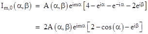
Now, any combination of these solutions will satisfy the original difference equation for nodes with zero net current, but we want I_0,0 = -1 Amp, and to achieve this we (again) take the absolute values of the indices, i.e., we define

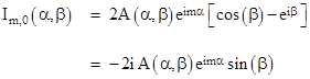
For values of m and n different from zero, taking the absolute values has no effect on the difference equation, i.e., it still gives zero net current. However, for m = n = 0 we get

This shows that if we put V_0,0 = 0 then for –1 Amp of current we must have V_1,0 = 1/4 volts, which is consistent with the fact that the resistance between two adjacent nodes of 1/2 ohms, because we superimpose this solution with an equal and opposite solution centered on the adjacent node with +1 Amp current.

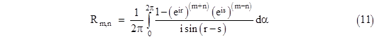
We don’t yet have a definite solution satisfying all the conditions, because with the absolute values of the indices we generally get non-zero currents for I_m,0 and I_0,n. To solve this problem, we will simply superimpose several of these solutions, and impose the requirement that the net currents of the form I_m,0 and I_0,n all vanish. To do this, we integrate the solutions of the form (4) over α ranging from –π to π. Thus we have

with the understanding that β is given as a function of α by equation (3). We will find that this determines the function A(α,β). Consider first the requirement I_m,0 = 0. Inserting the expression for V_m,0 from equation (4) into equation (1), we have, for all m > 0,

Making use of the characteristic equation (3), this can be written as

Now we seek to superimpose many of these solutions such that the net current for these expressions is zero. To do this, we will integrate this expression over α ranging from –π to π. Thus we have

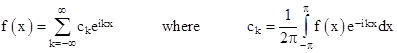
At this point we recall that the exponential Fourier series for an arbitrary function f(x) is

Therefore we have

where we’ve made use of the fact that I_0,0 = -1 and I_m,0 = 0 for all m ≠ 0. From this we infer that

Inserting this into equation (5), we get

Again, it’s understood that β is given as a function of α by equation (3). It might seem as if we cannot now force the currents I_0,n to equal zero. If we had imposed that requirement first, instead of I_m,0 = 0, by symmetry we would have found

which seems superficially different from (7). However, notice that the limits of integration are reversed, because α and β progress in opposite directions. Furthermore, if we take the differential of the characteristic equation (3) we get

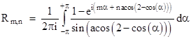
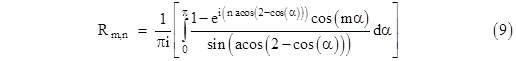
which proves that (7) and (8) are equivalent. As discussed previously, the resistance between the origin and the node (m,n) is twice the value of V_m,n - V_0,0, so we have the formula

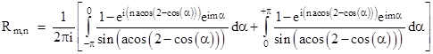
This can be split into two integrals, one ranging from –π to 0, and the other ranging from 0 to +π, as follows:

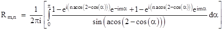
Reversing the sign of α in the first integral, and noting that cos(–α) = cos(α),  this can be written as

and hence we have

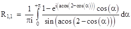
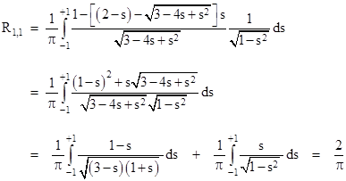
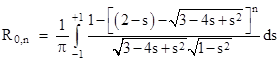
For example, the resistance between two diagonal corners of a lattice square is given by

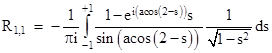
If we define the variable s = cos(α) we have α = acos(s) and

As α ranges from 0 to π, the parameter s ranges from 1 to –1, so the preceding integral can be written as

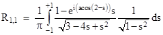
We now make use of the identity

to re-write the integral as

Also, from the identity

we have

so the integral can be written as

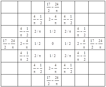
(This same result can be derived purely algebraically, without the use of Fourier series, as described in another note.) Knowing this resistance value for diagonal nodes, and the resistance value 1/2 for adjacent nodes, we can immediately compute the resistances to several other nodes by simple application of the basic difference equation. Thus we have the resistances relative to the origin shown below.

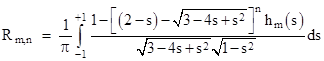
Returning to equation (9), we see that the same substitutions and identities that we used to simplify R_1,1 enable us to write the general expression as

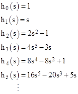
where h_m(s) denote the trigonometric polynomials giving cos(mα) as a function of s = cos(α). The first several of these polynomials are

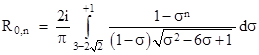
The coefficients of these polynomials are given by a simple recurrence relation, and they also have a simple trigonometric expression. However, we don’t actually need to deal with these polynomials, because it is sufficient to determine the values of R_0,n by the above integral, and then all the remaining resistances are easily determined by simple algebra. Hence we can focus on just the integrals

To simplify this still further, we can define the parameter

in terms of which s and ds are given by

Re-writing the expression for R_0,n in terms of the parameter σ, we get

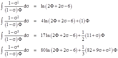
Making use of the indefinite integrals

where

we can determine the values

and so on.

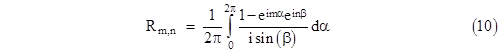
Another way of simplifying the integrals involved in the infinite grid solution is to return to equation (7), focusing on the case of positive m and n with m > n, and recalling that the resistance from the origin to the node (m,n) is twice the voltage given by (7), so we have

where, for convenience, we’ve shifted the limits of integration from the range [–π,+π] to the range [0,2π]. Now suppose we define new variables r,s such that α = r + s and β = r – s. Substituting for α and β in equation (3) gives the relation cos(r)cos(s) = 1. In terms of these parameters equation (10) can be written as

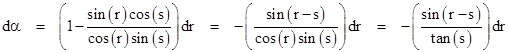
Obviously we have dα = dr + ds, and differentiating the relation cos(r)cos(s) = 1 gives

so we have

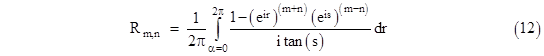
Making this substitution into (11) gives

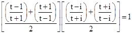
Now, since cos(r)cos(s)=1 where cos(z)=(e^iz+e^−iz)/2, and in view of the identity

we see that r and s can be expressed parametrically in terms of a single parameter t such that

From this we get

With these substitutions, equation (12) becomes

To this point we have continued to specify the limits of integration in terms of α, but now we note as α ranges over the real values from 0 to 2π we have t = (1–i)τ where τ is a real-valued parameter ranging from infinity to 0. Hence we make this change of variable to express the result as

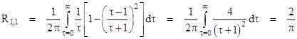
where we’ve made use of the fact that the variable τ can be multiplied by an arbitrary factor inside the curved parentheses without affecting the integral. For the first diagonal node we have m = n = 1 and the integral is simply

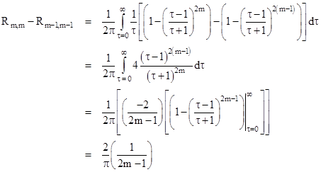
For the resistances to the other nodes along the diagonal of the lattice, notice that for any m we have

Consequently we have the well-known result

from which all the other resistances are easily computed using the basic recurrence relation (1). In another note we consider the same problem from a more algebraic standpoint.

Return to MathPages Main Menu