Generalizing Pythagoras and Carnot

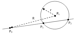
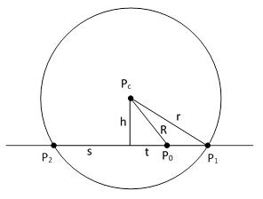
Consider a circle of radius r centered on the point P_c, and an arbitrary point P₀ at a distance R from P_c. We then draw a line through P₀ intersecting the circle in the points P₁ and P₂ as shown below.

The angles with which the circular locus cuts across the line at the points P₁ and P₂ are equal and opposite (i.e., complementary), so if we rotate the line incrementally about the point P₀, the lengths of the segments P₀P₁ and P₀P₂ will change at a rate always proportional to their current lengths, and these rates of change will have opposite signs. Letting L₁ and L₂ denote these two distances, we have dL₁/L₁ = −dL₂/L₂, which implies L₁dL₂ + L₂dL₁ = d(L₁L₂) = 0. Therefore, the product of these two distances is constant. To determine the value of this constant, we need only rotate the line so that is passes through P_c as shown below, and then note that the distances from P₀ to the points of intersection are R−r and R+r, so their constant product is R² – r².

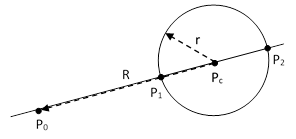
On the other hand, if we rotate the line so that it’s tangent to the circle, the points P₁ and P₂ coincide, both at a distance L from P₀, and the line from P_c to the point of tangency is perpendicular to the tangent line, as shown below. In this case our proposition gives the relation L² = R² – r², which is Pythagoras’ theorem.

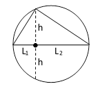
Thus the Pythagorean theorem L² = R² – r² can be seen as just a special case of the more general proposition L₁L₂ = R² – r². Incidentally, the same relation applies even if P₀ is inside the circle, provided we treat the lengths L₁ and L₂ as signed quantities depending on their direction from P₀. Since the product of the two distances from a point to the circle along any given line is constant, we can immediately infer the “hyperbolic” form of Pythagoras’ theorem, L₁L₂ = h², from the figure below, where the line along L₁ and L₂ is a diagonal of the circle. (By completing the rectangle, we can see that the upper vertex is a right angle.)

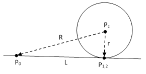
In Propositions 35 and 36 of Book III of Euclid’s Elements the proposition  L₁L₂ = R² – r²  is proved by mean of Pythagoras’ theorem, as shown in the figure below.

We drop the perpendicular h from P_c to the line P₁ P₂, and then note that the product of the segments P₀P₁ and P₀P₂ is (s−t)(s+t) = s² – t². Also, the Pythagorean theorem gives s² = r² – h² and t² = R² – h², so the product of our two line segments is r² − R². This is a nice proof, but it’s reliance on the Pythaogrean theorem prevented Euclid from placing it in Book I. Compare this with our previous proof, which consisted of the observation that as the line P₁P₂ rotates about P₀ the segments P₀P₁ and P₀P₂ vary at rates always proportional to their lengths, one increasing and the other decreasing, so their product is constant. Admittely this is essentially a calculus argument, which Euclid would probably not have considered acceptable, but it bears a strong resemblence to some of the arguments used by Archimedes several centuries later. If Euclid had found a way to prove this proposition with invoking his I.47, he could then have immediately proved I.47 based on this result.

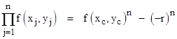
The proposition  L₁L₂ = R² – r²  represents an algebraic relation between a set of distances r, R, L₁, and L₂ defined in terms of orthogonal coordinate differences by the basic function

The distance between the points P_i and P_j is defined as f(x_i−x_j, y_i−y_j). Assigning the point P₀ to the origin of our coordinate system, we can express the proposition as

where P₁ and P₂ are the intersections of any line through the origin with the locus defined by f(x−x_c,y−y_c) = r.  Letting n denote the degree of the base polynomial (so n = 2 in this case), we can write this in the form

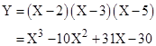
It turns out (as shown in the article on A Quadrilateral in a Circle) that this proposition is true for any arbitrary homogeneous polynomial f of any degree n in any number of variables. Also, we can convert any polynomial to a homogeneous one in a higher dimension. To illustrate, consider a simple cubic curve

This locus is not expressed in homogeneous form, but if we define X = x/z and Y = y/z we can substitute into this equation to give the homogeneous surface in three dimensions

We now define the function

On the plane w = 1 with u = X and v = Y this is our original cubic curve, so we choose the “center” point x_c = y_c = 0, z_c = −1, and consider the locus of points such that

On the plane z = 0 this locus is our original cubic. We choose to evaluate the intersections of this curve with the line through the origin with the slopes k_y = 0 and k_z = 0, so we know the intersection points are at x₁ = 2, x₂ = 3, and x₃ = 5. Noting that r = 0, the theorem gives us the relation

Both sides evaluate to 30, confirming the equality. It follows that if we tilt the line through the origin by setting ky to some non-zero value, the product of the f-functions of the coordinates of the three new points of intersection with our original cubic is always 30. Morevoer, we can tilt the line in the z direction by setting kz to some non-zero value, and still the product of the f-function of the coordinates of the three points of insection with the cubic surface is 30, even if we tilt the line to such an extent that the points of intersection have complex coordinates.

In a sense, the “f-function” serves as a kind of “distance” function, but of course it isn’t the literal distance, unless f happens to be the metric function

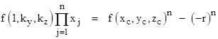
However, our proposition can still give us information about the relations between the literal distances. Consider the locus of points satisfying f(x−x_c,y−y_c,z−z_c) = r where f is an arbitrary homogeneous polynomial of degree n. Letting P₁, P₂,… P_n denote the points of intersection of the line given by y = k_yx, z = z_yx, we can write our basic proposition in the form

In general the left-hand side is not the product of the literal distances, but we can form the product of the literal distances if we simply divide by f(1,k_y,k_z) and then multiply by the metric function g(1,k_y,k_z). Thus we have

where L₁, L₂, … L_n are the literal distances from the origin to the points of intersection P₁, P₂, …, P_n. Obviously this product is not invariant because it depends on the slopes of the line, but the quantity in the square brackets is invariant for any given focal point in relation to the “center” of the locus. Thus the product of distances from a given focal point P₀ to a locus along a line with the slopes α,β can be factored as F(P₀)G(α,β) where the function F depends only on the focal point and the function G depends only on the slopes of the line.

Now consider a set of m arbitrary points, denoted by Q₁, Q₂, …, Q_m, and the cycle of m lines Q₁Q₂, Q₂Q₃, …, Q_mQ₁.  Let the slopes of the line from Q_j to Q_j+1 be denoted by α_j and β_j, and let ϕ_j,k denote the product of the literal distances from Q_j to the locus along the line from Q_j to Q_k. Then we have

Each of the points has another set of distances to the curve, taken along the other line passing through that point, and we can evaluate the product of those products as

Both of the above products consist of the same factors, so we have the relation for the products of the literal distances

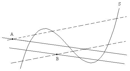
This corresponds to Carnot’s theorem on transversals, generalized to cycles of arbitrary length. We can immediately generalize it still further, because the relation applies not just to the products of the literal distances, but to the products of any homogeneous function of the coordinate differences. To see this, simply replace the metric function g with any other function. It also follows that the ratio of any function of the coordinate differences from any two given points to a curve along parallel lines (with arbitrary slopes) is invariant. So, for example, in the figure below, the product of the distances from A to S divided by the product of the distances from B to S is the same, regardless of whether the distances are evaluated along the two solid lines or the two dashed lines (or any other pair of parallel lines through the points A and B).

Return to MathPages Main Menu