Transfer Functions and Causation

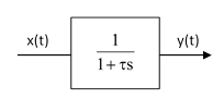
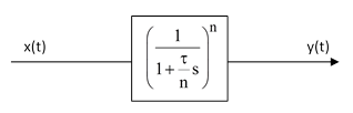
One of the most common transfer functions used in the modeling of dynamic systems is the simple first-order lag, usually depicted schematically as shown below.

The arrow conventionally signifies that y(t) is the dependent variable, driven by x(t), which is regarded as an independent variable. The symbol “s” is effectively a differentiation operator (see Laplace transforms), and we consider the transfer function as an operator that multiplies x(t) to yield the result y(t). We can express this formally as

Often we multiply through by 1 + τs to give

which represents the closed-form differential equation

For any given forcing function x(t) we can solve this equation for y(t). However, we can just as well expand the operator in (1) using the geometric series, and write it in the form

If we substitute this infinite series for y into (2), we can verify that it is consistent, assuming convergence, so equations (2) and (3) are compatible, but are they completely equivalent? Consider a simple example with x(t) = A + Bt for some constants A and B. If we substitute this for x(t) in equation (2) and solve the resulting differential equation we get the general solution

where C is an arbitrary constant of integration. On the other hand, if we insert x(t) = A + Bt into equation (3) we get simply

Thus it might seem as if (2) is more general than (3). In a sense we introduced the extra term Ce^–t/τ into the solution (4) when we multiplied through equation (1) by 1 + τs, which equals zero when applied to the function Ce^–t/τ. Another way of looking at the difference is to note that if x(t) equals A + Bt for all time, and if y(t) has been related to x(t) by the subject transfer function for all time, then indeed the only solution is (5). In contrast, the appearance of x(t) on the left side of equation (2) just represents the instantaneous value of the function at the time t, which leaves y(t) with a degree of freedom. One could also argue that the term Ce^–t/τ is similar to a gauge freedom. Recall that any solution of the equations for the potential of an electromagnetic field can be augmented by functions of an arbitrary scalar field. Similarly the particular solution of (2) can be augmented by any multiple of the homogeneous solution.

It’s interesting that equation (2) presents x as a linear combination of y and its first derivative, whereas equation (3) presents y as a linear combination of x and all its derivatives. So these two equations represent two different interpretations of the causal structure.

We also note that, according to equation (5), we have y(t) = x(t – τ), meaning that y is a delayed version of x. However, this is true only for the case when x is a linear ramp function (for all time). If x(t) is some other function of time, the relationship between x and y varies. Even for purely sinusoidal functions the amplitude and phase lag varies with frequency. Also, if we regard x as an independent input, any change in x has an instantaneous effect on y, albeit extremely attenuated. Thus a single first-order lag cannot represent an actual time delay such as is associated with propagation of a signal across a distance at a finite speed in accord with Huygens’ Principle.

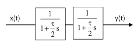
To more closely approximate a true time-delay transfer function, for a delay equal to τ, we could place two first-order lags in series, each with a time constant of τ/2, as shown below.

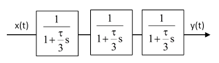
For an infinite ramp input, the output would be delayed by t, just as for the single transfer function, but the “early” response to a step change in x(t) would be significantly less, because it would have to elevate the output of the lag appreciably before it begins to elevate the output of the second lag. To make the delay even more sharp, we could place three lags in series, each with time constant t/3, as shown below.

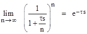
Continuing in this way, we can consider the limit of n lags in series, each with time constant τ/n, and evaluate the result in the limit as n increases to infinity. Multiplying all the transfer functions together, the series of n lags can be depicted as

Algebraically we have the limiting relation

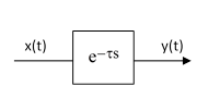
so we can represent this relationship between x and y by the transfer function shown below.

We claim that this gives y(t) = x(t – τ) for any input function x(t). In other words, the output is an exact replica of the input, but delayed in time by the amount τ. We already know this is true if x is a linear ramp, but what about a sinusoidal function? Written explicitly, the direct relationship provided by this transfer function is

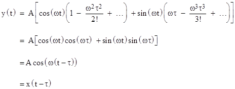
Now suppose x(t) = Acos(ωt) for some constants A and ω. Inserting this into the above expression gives

Grouping the sine and cosine terms, this can be written in the form

This confirms that the operator e^–τs represents a pure time delay not only for ramp functions but also for sinusoidal functions. Furthermore, recalling that we can express any arbitrary function as a Fourier series consisting of a sum of cosine functions of various amplitudes and frequencies, and that our differential equation is linear so solutions are additive, we see that the effect of this transfer function on any arbitrary input is to apply a pure time delay. The value of y at any time t is simply the value of x at the earlier time t – τ. This might seem to suggest that no information about what is happening to x at time t can be inferred from the value of y until the later time t + τ, consistent with usual notions of causality. However, as discussed above, a transfer function does not contain an implicit directionality, it is simply a relationship between two variables, and can just as well be regarded as giving x as a function of y, in which case we have x(t) = y(t + τ). Thus at any time t, the variable x has the value that y will have at the future time t + τ. This seems to conflict with our usual notions of causality, so it’s interesting to examine this point of view in detail.

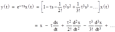
Let us write the relationship between x and y implied by this transfer function as

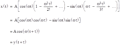
If we now treat y as the independent variable and consider the case y(t) = Acos(ωt) for some constants A and ω, we have

Grouping the sine and cosine terms, this can be written in the form

which confirms that this transfer function implies x(t) = y(t + τ). The advantage of writing the relationship in this explicit form is that it shows how x(t) depends not only on y(t) but also on all of its higher derivatives. In the context of perfectly continuous variables, knowable to infinite precision, we could in principle determine y(t) and all its derivatives from any non-zero range of the values of y(t), and hence we could compute x(t) by the above formula, which is y(t + τ), i.e., the future value of y(t). This should not be surprising, because, assuming y(t) is analytic we can express it as a power series

for constant coefficients y₀, y₁, …  By evaluating the derivatives at time t = 0, it’s easy to see that these coefficients are related to the derivatives of y according to

Thus by specifying the derivatives of y at any given time, we are specifying the entire function y(t) for all time. From this point of view, our transfer function is just an operation that, when applied to the value and derivatives of an arbitrary analytic function at a given time t, extracts the value of that function at the time t + τ. Of course, the stipulation that y(t) has a power series expression that applies for all time (or at least for the time up to t + τ) implies that the future of the y function is already determined and implicit in its present behavior. This is reminiscent of Laplace’s famous remark about how the entire history of the universe – assumed to follow fully deterministic and suitably simple laws – would be knowable at a glance to a being capable of perceiving the present condition with infinite precision. In practice, human attempts to extrapolate the future from the past and present have had mixed results. It’s conceivable that new information arises in the world from time to time, either by the exercise of free will, or by some kind of randomness (playing dice, quantum uncertainty, asymptotic sensitivity and functional singularities, etc.). It’s also conceivable that the future really is fully implicit in the present, as Laplace imagined, but that it is unknowable, due either to the necessarily finite amount of information we can access, or to limitations on the precision of our perceptions. (For more on this, see the note Is the World Provably Indeterminate?)

Another interesting aspect of transfer functions is their bi-directionality. As discussed above, we can regard either x(t) or y(t) as the independent variable, and the other as the dependent variable, so the flow of causation is ambiguous. If we were attempting to use a transfer function to represent the interaction between physical entities, this bi-directionality would seem suitable, since physical interactions entail mutual influence (every action has a re-action). However, the pure lag and delay functions we’ve been considering so far are asymmetrical in the sense that they are retarded in one direction and advanced in the other. For real physical interactions, according to the usual interpretation, we would expect retarded action in both directions. There are, of course, some theories that invoke both advanced and retarded interactions, but they should be symmetrical. This suggests that, rather than considering either x(t) = e^τsy(t) or y(t) = e^τsx(t), we might consider a symmetrical relationship of the form

This might seem to signify the identity mapping, but this equation has non-trivial solutions as well. Defining z(t) = x(t) – y(t), we can write this as

Thus we have a “relativistic theory”, in the sense that only the difference between x and y is physically significant. Also, it is a homogeneous theory, in the sense that all the dynamics are contained in the “left side” of the equation, and there is no external independent “forcing function” or “source term” on the right side. The presence of a source term in physical theories has sometimes been viewed as a deficiency, because it represents all the elements that are not comprehended by the dynamics of the “left side”. For example, regarding the field equations G_μν = T_μν of general relativity Einstein said “the right hand side is a formal condensation of all things whose comprehension in the sense of a field theory is still problematic”, and he hoped to ultimately eliminate this “unnatural” source term by absorbing it somehow into a more comprehensive notion of the field. Our transfer function can be seen as a simplistic example of a physical model with no source term, governed purely by the homogeneous equation

This equation has infinitely many different solutions, depending on the initial conditions. For example, we can specify the value and any finite number N of derivatives of z at the initial time t = 0, and then the only constraint on the remaining derivatives of z is that the above equation is satisfied. One of the infinitely many ways of doing this would be to choose the (N+1)th derivative so that it cancels all the preceding terms, and then set all the higher derivatives to zero. This would give a finite power series for z(t). Another way, for the same values of the first N derivatives, would be to select all higher derivatives to some non-zero values, subject to the constraint of the above equation. This shows that, even for a given set of low-order derivatives, the transfer function allows an unlimited number of different “futures”. For any given solution z(t), the future would be completely deterministic, but also completely unknowable based on observations with anything less than perfect precision. This equation evidently places no meaningful constraint on the solution z(t) in the absence of some other principle governing and restricting the initial conditions.

Return to MathPages Main Menu