Laplace Transforms

For any given function f(t) (assumed to equal zero for t less than zero) we can define another function F(s) by the definite integral

The function F(s) is called the Laplace transform of the function f(t). Note that F(0) is simply the total area under the curve f(t) for t = 0 to infinity, whereas F(s) for s greater than 0 is a "weighted" integral of f(t), since the multiplier e^–st is a decaying exponential function equal to 1 at t = 0. Thus as s increases, F(s) represents the area under f(t) weighted more and more toward the initial region near t = 0. Knowing the value of F(s) for all s is sufficient to fully specify f(t), and conversely knowing f(t) for all t is sufficient to determine F(s). Thus there is a unique "mapping" between functions in the "t domain" and the corresponding functions in the "s domain".

The usefulness of Laplace transforms is due to the fact that some problems which would be difficult to solve in the "t domain" are easy to solve in the "s domain". To see why, it's helpful to review some fundamental properties of these transforms. For any given function f(t) that is zero for all t less than zero, let L[f] denote the Laplace transform of f. The Laplace transform is a linear operator, which means that for any functions f,g, and constant c we have

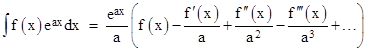
Now, the key to the usefulness of Laplace transforms arises from the following indefinite integral

which can easily be verified by differentiating the right hand side using the chain rule. From this integral, it follows that the Laplace transform of a function f(t) can be expressed as

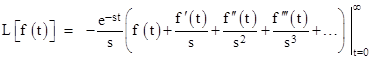
With t = +∞ the right hand quantity vanishes, so the Laplace transform is simply given by the negative of the indefinite integral evaluated at t = 0, i.e.,

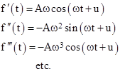
This makes it easy to see that if f(t) is a constant A, then L[f] = A/s. Also, if f(t) = At + B, then f ′(t) = A and the Laplace transform is L[f] = B/s + A/s². For a less trivial example, suppose f(t) = A sin(ωt + u) for some constants A, ω, and u. This function has the derivatives

Substituting these derivatives, at t = 0, into equation (2) gives

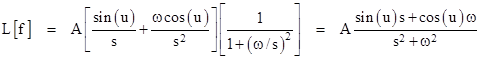
Collecting terms by sines and cosines, this can be written as

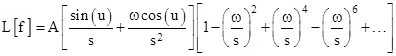
The right-hand factor is just a geometric series in –(ω/s)², so we have

In the special case when the phase angle u is zero, this reduces to the familiar result L[Asin(ωt)] = Aω/(s² + w²).

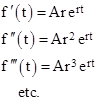
Another useful example is f(t) = Ae^rt for constants A and r, which has the derivatives

Thus by equation (2) we have the Laplace transform

Similarly the Laplace transform of the function

is given by

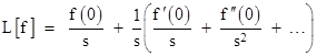
So, we've seen how equation (2) enables us to determine the Laplace transforms of typical functions, but the most important point to notice about (2) is that it can be written in the form

and the quantity in parentheses is L[f ′]. Therefore, rearranging terms, we can write this as

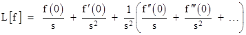
By the same token we could write (2) as

and, noting that the quantity in parentheses is L[f ″], we can multiply through by s² and rearrange terms to give

Likewise we can deduce

and so on. In this way we can express the Laplace transform of the nth derivative of f(t) as a polynomial in s with coefficients given by the derivatives of f(t) at t = 0 and a leading coefficient of L[f]. To see how this can be used to solve differential equations, consider the homogeneous equation

In order to determine a particular solution for this 2nd-order equation we must specify two conditions. Often we are able to specify the "initial conditions", i.e., the values of f(0) and f ′(0). So, taking the Laplace transform of both sides of our differential equation (recalling that L is a linear operator), we have

Substituting the previous expressions for the transforms of these derivatives, we have

Collecting terms, this gives

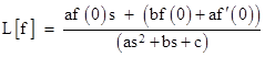
Solving for L[f] gives

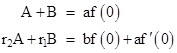
We recognize this as the Laplace transform of Aexp(r₁t) + Bexp(r₂t) where r₁,r₂ are the roots of the characteristic equation in the denominator of the right side, and A,B are constants satisfying the conditions

Thus for any coefficients a,b,c we can determine the characteristic roots r₁,r₂, and then for any given initial conditions f(0) and f ′(0) we can solve for A and B to give the complete solution. This example was based on a homogeneous equation, i.e., an equation with no forcing function, but Laplace transforms can also handle inhomogeneous equations, simply by taking the transform of the forcing function along with the other terms of the equations, and then solving for L[f] just as above.

We can also deduce several other interesting facts about Laplace transforms from equation (2). For example, it's easy to show that if L[f(t)] = F(s), then

Although Laplace transforms are certainly interesting, and can be useful in some circumstances, they also have some drawbacks. Most obvious is the fact that they require "initial" conditions, i.e., we must stipulate the value and derivatives of f(t) at t = 0, whereas we often wish to impose conditions at different points of the function, such as specifying f(1), f ′(3), and f ″(17). These three conditions are just as suitable for fixing the solution of a 3rd-order differential equation as are f(0), f ′(0), and f ″(0), but since they are imposed at different values of the independent variable we cannot use the conventional Laplace transform method.

Another drawback of Laplace transform methods is that they tend to be taught as a "canned" technique, enabling one to solve equations by a simple recipe, without really understanding how it works. The problem with this approach is that it can easily give erroneous results if applied inappropriately. It's also worth noting that any equation that can be solved by Laplace transforms can also be solved (often more efficiently and perspicuously) by other methods.

Return to MathPages Main Menu