Electrodynamics - The Curl of the Curl

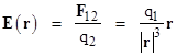
Coulomb’s law expresses the electric force between two stationary charged particles. If a charge q₁ is at rest at the origin of a system of inertial coordinates x,y,z, and q₂ is at rest at the position r, the exerted by q₁ on q₂ is

If the charges have the same sign, the force is positive, meaning that it tends to push q₂ away from the origin, whereas if the charges have opposite signs the force is negative, meaning it tends to pull q₂ toward the origin. The contribution of q₁ to the electric field E at the position r is defined as the force per unit charge, so we have

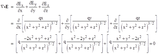
This is a purely central force, i.e., the force vector points directly toward (or away from) the source charge, so the components E_x, E_y, E_z of the electric field E are proportional to the components x,y,z of r. If r is not zero, the divergence of E is identically zero, as shown by

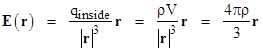
The vanishing of the divergence applies to all charge-free points in any central inverse-square vector field, and to any linear combinations of such fields. To cover the regions in which charge is present, suppose the charge q is distributed uniformly with density r in a sphere centered on the origin. By Newton’s lemma, we know that for any point outside the sphere we can treat the field as if the charge was all concentrated at the origin, and for any point r inside the sphere we can ignore the charge at a radius greater than r, and treat the charge at a radius less than r as if it was all concentrated at the origin. The volume of a sphere of radius r is V = (4/3)π|r|³, so for interior points the electric field is given by

and therefore the divergence is

Thus in general we have

In physical terms this signifies that the integral of the electric flux over any closed surface equals the charge enclosed in that surface (Gauss’ Law). In fact, if charge is to be conserved, this equation must be true in all conditions, not just for stationary arrangements of charges. Hence this is taken as one of Maxwell’s equations for the electromagnetic field. However, even though every central inverse-square force field satisfied this equation, not every solution of this equation corresponds to a central inverse-square force field (nor a linear combination of such fields).

For any arbitrary vector field K it can be shown that the divergence and the gradient don’t commute. Specifically, we have the identity

Consequently if we take the gradient of the divergence of the electric field in a region of uniform charge density (possibly zero), and note that the second term on the left side of the above identity is the Laplacian, we get

The second term on the left side is the curl of the curl of the electric field. Now, if E is a central isotropic field, it is of the form E = [xf(r), yf(r), zf(r)] and the x component of the curl of E is

Similarly the y and z components are zero, so the curl of any isotropic central force field (or linear combination of such fields) vanishes. Consequently, in any region of uniform charge density, and assuming E produces an isotropic central force, the field equation is simply

The only places where this equation would not hold is on the boundary of regions of uniform charge density. It can be shown that for any set of boundary conditions equation (3) uniquely determines a solution E for the entire space. Thus it unambiguously determines the electric field for any stationary configuration of charges. However, it’s clear that this equation cannot be valid for charge configurations that are changing as a function of time, because it implies that the field at every point in space responds instantaneously to any changes in the charge configuration, thereby allowing faster-than-light signaling. Hence we know (3) is not covariant under Lorentz transformations. It follows that in dynamic conditions E must not be an isotropic central field, because the curl of the curl of E must not be zero, and we must revert to equation (2) for these time-dependent conditions.

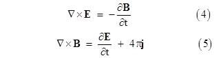
Since equation (2) has no explicit time-dependence, it might seem as if, like equation (3), it predicts instantaneous response to changes in the charge configuration. However, unlike equation (3), it can be shown that equation (2) does not uniquely determine the electric field E for a given spatial configuration of charges. In order to determine the electric field in the presence of moving charges we need additional information. Specifically, we need to know how the curl of the curl of E varies in response to moving charges. This additional information is supplied by two more “Maxwell equations”. These equations involve an auxiliary vector field B, called the magnetic field, as follows

The symbol j denotes current density, which is zero in empty space. If we take the curl of both sides of (4) we get

Substituting for the curl of B from equation (5), with j equal to zero, we find that

Thus Maxwell’s equations imply that the curl of the curl of E is the negative of the second partial derivative of E with respect to time. Substituting into equation (2) gives the general field equation (for points where the current density is zero, and not on the boundary between regions of different charge density)

We recognize this as the wave equation, and it is straightforward to verify that it is covariant under Lorentz transformations. Also, it implies that changes in the electric field propagate at a characteristic speed. This speed is the square root of the reciprocal of the coefficient of the second term in (6), which is the ratio of electro-static to electro-magnetic units. We have chosen to work in units such that the electric permittivity and the magnetic permeability are both 1, so the characteristic speed is unity, but if we revert to conventional units the coefficient of the second term in (6) is the product μ₀ε₀ where μ₀ and ε₀ are the permeability and permittivity of the vacuum. Thus the speed at which changes in E propagate (in vacuum) is

Returning to the static case, when the curl of E is zero, it follows that a static E field is conservative, i.e., the net work required to move a test charge quasi-statically from one point to another is independent of the path that is followed, so if the particle is returned to its original position the net work is zero. For a conservative field we can define a potential function for each point in space, such that the difference between the values of the potential at two points equals the work required to move quasi-statically from one point to the other. For an incremental movement in the x direction the work done is dϕ = –E_xdx, which implies that E_x = –∂ϕ/∂x, and likewise for the other components, so we have

for an electrostatic field. Substituting into equation (1) gives

Thus for a given stationary configuration of charge density we can determine the unique potential field (with the convention that the potential is zero at infinity). The contribution to the potential at a given location of a point charge q located a distance r away is simply q/r, and the total potential is just the sum of the contributions for all charges. However, it’s important to bear in mind that this applies only to quasi-static motions in a static electric field, as is clear from the fact that the potential equation has no time-dependence. Furthermore, equation (7) is inconsistent with Maxwell’s equation (4), because the curl of the gradient of any scalar field is identically zero, so equation (7) implies that the curl of E vanishes, whereas we know from equation (4) that the curl of E equals the negative of the partial derivative of B with respect to time.

This suggests that the correct form of (7) for dynamic conditions must include another term on the right hand side whose curl is the time derivative of B. In other words, we need a vector field A such that

and then the electric field can be written as

Taking the curl of both sides of this equation gives (4), as required. Thus, Maxwell’s equations imply that a single scalar potential is not adequate to represent the electromagnetic field. In dynamic conditions we need a vector potential A as well.

If we now take the divergence of (10) and re-arrange terms we get

Substituting from (1) into the right hand side and reversing the order of differentiation in the second term on the left gives

At this point it’s worth pointing out that the potentials ϕ and A are not unique for given fields E and B. As mentioned previously, the curl of the gradient of any scalar field is zero, so equation (9) would be unaffected if we incremented A by the gradient of an arbitrary scalar field Ω. Then in order to leave (10) unaffected we would need to decrement ϕ by the partial derivative of Ω with respect to time. Thus if the potentials ϕ and A give the electromagnetic fields E and B, then exactly the same electromagnetic fields are given by the potentials

The scalar field W is arbitrary, since it has no effect on the observable fields. This is called a gauge transformation, and we can choose whatever gauge is convenient. For example, if we wish, we could set Ω = ϕ, which shows that we can stipulate ϕ = 0, and then we would only need to deal with the vector potential. However, it is often more convenient to adopt a different gauge. Notice that if we take the divergence of the A gauge transformation and the partial derivative with respect to time of the ϕ gauge transformation we get

Adding these two equations together gives

For any given potentials A and ϕ we can force the left hand quantity to equal zero by choosing a gauge transformation with the scalar field Ω satisfying the equation

Therefore, without loss of generality we are free to impose the gauge condition

This is often called the Lorenz gauge, after the Danish physicist Ludwig Lorenz (not Hendrik Lorentz). Incidentally, even after we impose this gauge condition, the gauge is still not uniquely defined, because the preceding equations show that the gauge condition is unaffected by adding to Ω any scalar field whose d’Alembertian vanishes. This degree of freedom corresponds to the unobservable phase of the quantum wave function of the system, and the gauge symmetry leads to conservation of electric charge in accord with Noether’s theorem.

Substituting the Lorenz gauge condition into equation (11) gives the correct field equation for the scalar potential

Like the equation for E, this is manifestly Lorentz covariant, and it shows that changes in the scalar potential propagate at the speed of light. Similarly we can find the field equation for the vector potential A by taking the curl of (9) and then making use of (5) to give

Substituting for the curl of the curl of A using the identity discussed previously and re-arranging terms, we have

If we take the partial derivative of (10) with respect to time, and substitute the resulting expression for ∂E/∂t into the above equation we get

Using the Lorentz gauge, the first two terms on the right hand side cancel, and we are left with the field equation for A

confirming that changes in the electromagnetic field propagate at the speed of light.

Return to MathPages Main Menu