Newtonian Precession of Mercury’s Perihelion

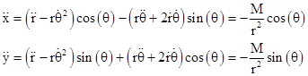
Given a large spherical gravitating body of mass M and a small test particle at a distance r, the Newtonian equations of motion imply that the test particle undergoes an acceleration of magnitude M/r² in the direction of the gravitating body, and no acceleration in the perpendicular direction.  (We are using units such that the gravitational constant and the speed of light are both unity.)  The test particle will be confined to a single plane, so its position as a function of time can be expressed in terms of the radial magnitude r(t) and an angular position θ(t) as

The second derivatives of these coordinates are

Since the absolute value of θ is arbitrary, these equations are equivalent to the conditions

Multiplying through the right hand equation by r, we have

and therefore the quantity in parentheses is constant, i.e.,

This represents the conservation of (specific) angular momentum, and it applies to any central force law, because such a force imposes no torque on the system. The constancy of this quantity also accounts for Kepler's second law, because the incremental area swept out by the position vector in an incremental time is dA = (1/2)r²dθ.

Making the substitution dθ/dt = h/r² into the left hand equation (1) gives

Notice that for a circular orbit all the derivatives of r vanish, and this equation reduces to h² = rM.  Making the substitution h = r²ω where ω = dθ/dt, we have ω²r³ = M, in accord with Kepler's third law.

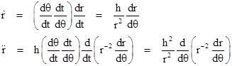
We can also use the relation dθ/dt = h/r²  to express the derivative of r with respect to time in terms of the derivatives of r with respect to the angular position θ.  We have

Inserting this expression for the second derivative of r into equation (2) and simplifying gives

Notice that the quantity in parentheses is just the negative of the derivative of 1/r with respect to θ.  Therefore, letting u = 1/r, we have the simple harmonic equation

In general the solution of an equation of the form

for constants Ω and p can be written in the form

where k is a constant of integration.  In the present case we have Ω = 1 and p = h²/M.  Recalling that r = 1/u, the path of the test particle in the gravitational field of a spherical body of mass M is

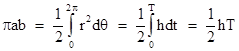
If the magnitude of k is less than 1, this is the polar equation of an ellipse with the origin at one focus (Kepler's first law), and with semi-latus rectum p = h²/M.  Now, the total area A of an ellipse with the major and minor semi-diameters a and b is πab, and this area can be expressed in terms of the integral

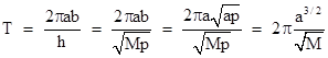
where we have made use of the fact that r²dθ = hdt.  Hence we have

which of course is Kepler's third law, M = ω²a³.  Thus we've reproduced Kepler's three laws for stable elliptical orbits of test particles around a perfectly spherical gravitating mass.

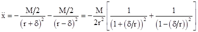
However, in actual physical situations, the gravitating body may not be exactly spherical.  For example, if the central body is spinning about its axis, it will be slightly oblate.  In such a case, the Newtonian gravitational field is not spherically symmetrical, and the force exerted on a test particle at a distance r is not exactly proportional to M/r².  As a result, the actual orbit of a test particle in such a case will not be exactly Keplerian.  To see how the effects of a non-spherical source, suppose the mass M is split into two spherical objects on the x axis separated by a distance 2δ.  The acceleration of a test particle located (also on the x axis) at a distance r from the center of mass of these two bodies is

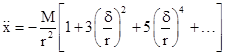
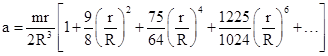
Since δ is small compared with r, we can expand the expression in square brackets to gives

Thus the predominant term in the acceleration is still inversely proportional to the square of r, but we now have a component inversely proportional to the fourth power of r, and another inversely proportional to the sixth power of r, and so on.  The non-Keplerian effects for a slightly non-spherical source can be inferred from just the first two terms.  Instead of (2), the radial equation of motion is now of the form

where J is a constant related to the oblateness of the gravitating body.  Repeating the previous transformations, we arrive at

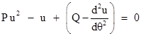
This is a non-linear equation, but can treat it as a quadratic in u of the form

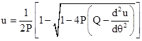
Solving this algebraically for u gives

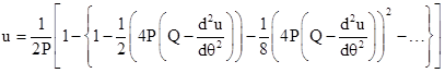
The second term inside the square root is much less than 1, so we can closely approximate the solution using just the first couple of terms of the expansion, so we have

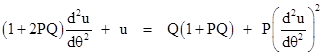
Simplifying and re-arranging terms, we get

The last term on the right hand side is negligible small, so we essentially have an equation of the form (3) with

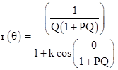
Hence the orbital path is described by the relation

This again is the equation of an ellipse, except that the period of the radial function is not exactly equal to the period of the angular position θ.  The angular travel necessary to go from one apogee to the next (for example) is not 2π, but rather 2π(1+PQ).  Hence the ellipse precesses by the amount 2πPQ radians per revolution.  In the case of our oblate gravitating body we have P = MJ/h² and Q = M/h², so the orbit precesses by 2π(M/h²)²J radians per revolution. 

Incidentally, if J = 3h² (corresponding to a term equal to h²/r³ in the potential) this gives the same precession as general relativity predicts for a perfectly spherical gravitating body.  Of course, the quantity h is specific to the particular orbit in question, whereas J is a fixed characteristic of the gravitating body, so it is not possible to replicate the relativistic precessions of more than one planet by hypothesizing solar oblateness.  In order to duplicate the relativistic prediction it would be necessary to hypothesize a gravitational potential that is dependent on the angular velocity of the test particle, not just on its position.

It's worth noting that although the actual oblateness of the Sun is believed to be negligibly small, the relativistic precession is still just a small fraction of the overall precession for a planet such as Mercury.  This is because the simple two-body Keplerian orbit is disturbed by the presence of gravitating matter outside the orbit.  For example, the orbit of Mercury precesses by about 532 seconds of arc per century due to the disturbing effects of the other planets, primarily Venus, Earth, and Jupiter.  (The French astronomer Urban LeVerrier in 1859 computed a slightly lower value of 526.7.) Even though these effects are strictly Newtonian, the calculations are far from trivial, especially for the effect of Venus. However, with certain simplifying assumptions we can derive a simple formula that gives results surprisingly close to those given by much more rigorous analyses.

The orbital periods of the planets are not synchronized, so over the course of many orbits their angular relationships will be averaged out.  On this basis, we might make a rough estimate of the perturbing effect of an outer planet (like Jupiter) on the precession of Mercury's orbit by imagining that the mass m of Jupiter is distributed uniformly in a ring around the Sun with a radius equal to the radius R of Jupiter's actual orbit.  Now, this is admittedly a rather dubious assumption, because the planet Mercury circles the Sun many times while a planet such as Jupiter has moved only a small angular distance. Thus one would think that a more representative model would treat the outer planet as essentially stationary, giving a dipole field. Note that, when Mercury and Jupiter are on the same side of the Sun, the gravitational pull of Jupiter acts in opposition to the Sun’s pull, whereas when Mercury and Jupiter are on opposite sides of the Sun, the effect of Jupiter is to pull Mercury more strongly “inwards” toward the Sun. In contrast, a uniform ring of matter always exerts a net outward pull on an interior planet. In view of this, the representation of the outer planets as uniform rings is certainly questionable, but it has the advantage of being fairly easy to evaluate, so using the “logic of the street lamp”, we will carry out the analysis based on the ring model.

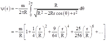
As discussed in Gravity of a Torus, the gravitational potential inside (and in the plane of) a ring of mass m is

and the acceleration (per unit mass of a test particle) inside such a massive ring (in the plane of the ring) at a distance r from the center is

directed radially outward from the center. (Incidentally, the same expressions arise in a completely different context, when evaluating the electrical resistance between two diagonally neighboring nodes of an infinite grid of resistors, as discussed in another note.) Hence we have an outward acceleration superimposed on the inverse-square acceleration inward toward the central gravitating body of mass M.  The radial equation of motion is therefore

where

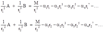
and so on. For small eccentricities the range of r values that must be covered is fairly small, and we can represent the right hand side of (5) by a more tractable form. Letting r₁ and r₂ denote the minimum and maximum radial distances of Mercury from the Sun, we seek constants A and B such that

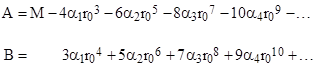
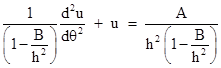
Solving this for A and B, letting r₀ denote the mean orbital radius of the test particle, and assuming very small eccentricity, we can re-write equation (5) approximately as

where

which can also be written as

Transforming back to the u parameter as before, this becomes

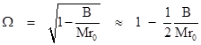
Using the fact that h² is approximately equal to Mr₀, and expanding the coefficient of the leading term, we see that the angular factor is

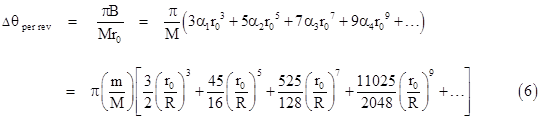
Subtracting this from 1 and multiplying by 2π, we get the approximate orbital precession per revolution due to a uniform ring of mass m and radius R.  This gives the formula

This gives the precession in units of radians per revolution of Mercury. To convert this to units of arc-seconds per century, noting that Mercury completes 414.9 revolutions per century, we multiply the above expression by

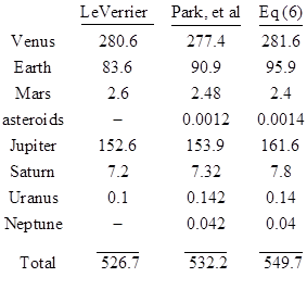
The table below shows the contributions to the precession of Mercury's orbit due to each of the next six planets as computed by LeVerrier, along with a more recent analysis (Park, et al, 2017), and as given by the above formula. The table also includes the contributions of the asteroid belt and the planet Neptune, neither of which were included in LeVerrier's analysis (presumably because he considered them negligible). The values listed are in units of arc seconds per century.

Evidently the crude approximation represented by equation (6) based on the dubious “ring” model somewhat over-estimates the correct values, but the results are surprisingly close to those given by more sophisticated analyses. Presumably LeVerrier's calculation of the Earth's contribution included the mass of the Moon, which is about 1.2% of the Earth's mass.  This represents roughly 1 second of arc per century.  Apparently his calculations did not include the asteroids, which contribute only about 0.0012 seconds of arc per century.  There are also a number of "Earth-crossing" asteroids that would have been omitted from LeVerrier's calculation. Some of these have such highly elliptical orbits that the circular ring approximation is probably not suitable.

The method of approximating the Newtonian planetary precession by modeling the planets as mass rings has been used in the literature, although no rigorous justification for it has been presented (to my knowledge). One example is a 1979 paper by Price and Rush, in which they not only use the mass ring model, they also make use of a slightly simplifying approximation by neglecting the angular offset of Mercury from the center of the solar system. (See their note 11.) The net effect of the bias due to this simplification, combined with the bias resulting from the use of the mass ring model, is to yield an incredibly good agreement with the more sophisticated methods. They calculate a total Newtonian precession of 531.9 arcseconds per century, essentially in perfect agreement with the best modern theoretical value of 532 – but this close agreement is spurious, since it results from two errors that just coincidentally happen to cancel each other. When the mass ring model is evaluated exactly, with no simplifying approximations (as we’ve done above), it yields nearly 550 arcseconds per century. The observed precession is 575, so even our crude approximation suggests that Mercury exhibits a bit more precession that we would expect based on Newtonian theory, but it only indicates about 25 arcseconds per century extra precession, whereas the best theoretical value raises this to 43. For a derivation of this extra precession from general relativity, see the note on Anomalous Precession. For a historical account of Einstein’s solution method, see the note on Conquering the Perihelion.

Return to MathPages Main Menu