An Infinite Series for Resistor Grids

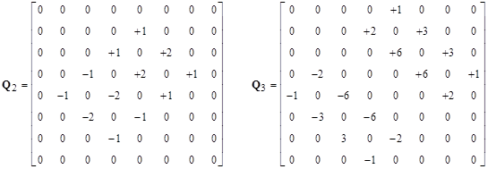
In another article we discussed the problem of determining the limiting value of resistance between two diagonally neighboring nodes of an square grid of unit resistors as the size of the grid increases toward infinity. We showed by means of somewhat subtle integrations how to derive the well-known result that the resistance approaches the value 2/π. In this note we show, by algebra, how to express this limit as an infinite series, and then how to prove that this series converges on the value 2/π. The series converges very slowly, but it has a very simple and appealing form, and we show that the same series arises in relation to the gravitational field of a ring of mass.

We begin with the fact that the net current p_i,j flowing out of the node [i,j] is

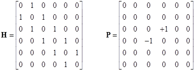
where V_i,j is the voltage at the node [i,j]. We place the voltages into a square array V of size N x N, and assume the voltages outside this square region are zero. Also, we assume the net current from each node is zero, with the exception of two diagonally neighboring nodes near the center of the square region. At those two nodes we have +1 unit of current flowing into one, and flowing out of the other. On this basis, all the equations of the system can be combined into the single matrix equation

where, with N = 6 for example,

Beginning with V = 0, we can iterate equation (2) recursively to converge on the solution. Of course, for small values of N we will soon encounter the effects of the boundary conditions, but for an arbitrarily large array we can forestall the boundary effect indefinitely. Thus we need only consider the pattern that emerges prior to encountering the boundaries.

Putting V₀ = 0 and letting V_n denote the nth iterate of (2), we find by simple substitution that

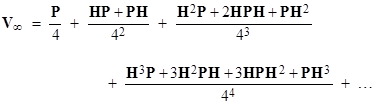
and so on. Thus as n goes to infinity the matrix V_n goes to

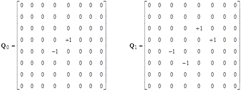
Letting Q₀ = P, Q₁ = HP + PH, and so on, the first several of these matrices (with N=8) are shown below.

The next iteration would extend beyond the boundary, but we can simply increase the size of the square region under consideration to N = 10, and we get the result

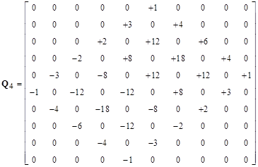
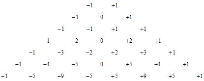
The pattern is clear. In each case the non-zero terms of Q_n consist of diagonals whose values are multiples of the nth row of binomial coefficients. Thus the diagonals of Q₄ consist of multiples of the quantities 1, 4, 6, 4, 1. The multipliers of these diagonals for Q₄ are -1, -3, -2, +2, +3, +1. If we arrange the multipliers for each of the Q arrays, we get the triangle

The terms of this array are given by the same recurrence as are the binomial coefficients, i.e., each number is the sum of the two numbers above it. Now, to determine the resistance between the two central diagonal nodes we must find the voltages for those nodes. The matrices Q_n for odd n don’t contribute anything to the sums for those terms, whereas for even n we get the contribution consisting of the middle binomial coefficient

multiplied by the “central” multipliers from the triangular array above. It’s easy to see that these multipliers are 1, 2, 5, 14, 42, and so on, i.e., the Catalan numbers

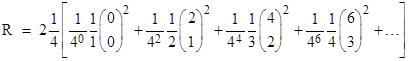
The total voltage between the two diagonal neighboring nodes is twice the magnitudes of the individual voltages, so combining the above facts we find that the net resistance between the two diagonally neighboring nodes is

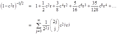
We can write this more perspicuously as

We can evaluate this summation numerically by noting that the initial term is s₀ = 1 and the subsequent terms are given by

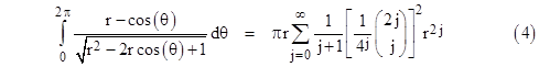
However, the series converges quite slowly. To evaluate the sum of this series analytically, note the definite integral

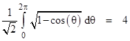
This can be found by expanding the integrand into a series in r, and then integrating the result, term by term. Now, with r = 1 the left hand side reduces to

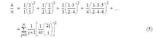
Substituting this into the previous equation with r = 1, we get the result

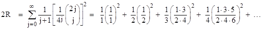
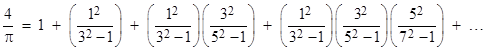
Since this quantity equals 2R we have R = 2/π, as expected. This series for 4/π can also be written in the form

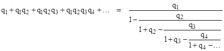
We can use this series to construct a continued fraction for π. Recall the following general relation between series and continued fractions

In view of the preceding expression we can set

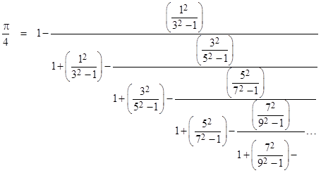
Taking the reciprocal of the above continued fraction, we have

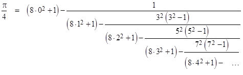
Clearing some of the fractions, this can also we written in the form

Oddly enough, the series involved in these expressions also arises in relation to the gravitational field of a mass ring. See the note on The Gravity of a Torus for more on this. It’s remarkable that the same series occurs in two such different contexts.

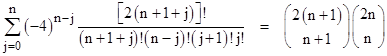
In our derivation of the identity (5) we somewhat glossed over the proof that the coefficients of the trigonometric integral expansion actually do have the closed form expression indicated in the summation. This amounts to proving the combinatorial identity

which is not self-evident. For a more tractable approach, consider the series expansion

It is relatively straightforward to determine the succinct closed-form expression for the expansion coefficients. Letting c denote cos(θ), we begin by expanding the integrand into a power series in r using the simple binomial expansion to give

Now we can integrate this, term by term, from θ = 0 to π, by making use of the well-known indefinite integral

From this it follows that

Therefore, we have rigorously established that the coefficients of the expansion (6) are

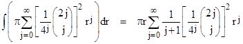
Now if we integrate the right hand side, term by term, we get

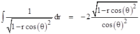
which has the same coefficients as equation (4), except that the exponent on r inside the summation is just j rather than 2j. To determine the value of this summation at r = 1, we can formally integrate the integrand of the left hand side of (8) with respect to r, giving the expression

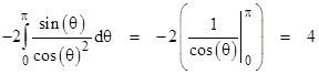
Setting r = 1 and formally integrating with respect to θ, we get

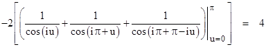
Thus integrating both sides of (8) with respect to r, and dividing through by π, we confirm the closed-form of the coefficients in the infinite series (4) for 4/π. However, there is a subtlety here, because the integral above doesn’t actually converge. This is why we referred to the above integration as formal, since it actually represents a divergent series. The basis of this type of formal manipulation is analytic continuation. Allowing θ to be complex, we can integrate from 0 to π over any simple path in the complex plane that does not pass through a singularity. For example, integrating along the straight segments from 0 to iπ to π+iπ to π we get

Likewise it can be shown that equation (7) remains valid when the integration is performed along this same piece-wise path that does not pass through any singularity. Thus our direct integration is really just formal shorthand for this more elaborate derivation.

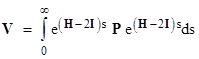
By the way, returning to equation (2), notice that it can also be written in the form

The solution is then given by inverting the commutation operator, which can be expressed by the well-known formula

This shows again the close similarities between the mathematics of resistor grids and of quantum mechanics, in which the commutation operator also plays a central role.

Return to MathPages Main Menu