The Dirac Delta Function

For any real numbers a,b with a < b, let S_a,b(x) denote a selection function, defined as

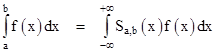
Using this function we can express the integral of a function f(x) over the range from x = a to b as follows

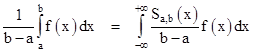
Thus, instead of specifying the range of interest by imposing explicit limits on the integration, we can formally integrate over all real values of x, using the multiplier S_a,b(x) to select the desired range. The total integrand equals 0 outside the specified range, and f(x) inside the specified range. The average value of the function f(x) from x = a to b is given by dividing the above integral by the length of the interval, i.e.,

If the values of a and b are extremely close together, the length of the interval approaches zero, and the average value of the function over that interval approaches f(a). Putting b = a + ε,  notice that we can always set a = 0 by simply shifting the argument of the selection function by a, so we have

It’s often convenient to consider this scaled selection function in the limit as ε goes to zero. In this limit we have

This leads us to define the so-called Dirac delta “function” as follows

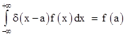
Strictly speaking this isn’t an actual function, because it is zero everywhere except at x = 0, where it is infinite. However, the symbol δ(x) may be regarded as useful shorthand for writing certain limiting cases of integrals. By definition, the integral of δ(x) over any range containing x = 0 is equal to 1, and the integral of δ(x) over any range not containing x = 0 is equal to 0. Also, the delta “function” has a well-defined effect when it appears in the integrand of any integral. For example, we can write equation (1) without explicitly referring to the limiting operation as

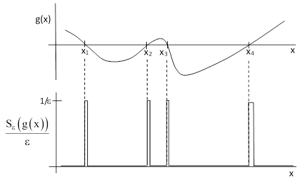
It’s often useful to be able to form the composition of the delta function with some other function. In general, consider δ(g(x)) where g(x) is an ordinary function with n distinct roots x₁, x₂, …, x_n. This means that g(x) = 0 for each of these n values of x, so these are the places where S_ε(g(x))/ε contains a spike, as depicted below for a function with n = 4 roots.

Notice that the widths of the spikes are not all the same in this view, even though this is drawn for a single fixed value of ε. The reason is that the argument of S is g(x), whereas we have plotted against x. The ε limit for the selection function is an increment of g rather than of x. Increments of g are related to increments of x by the derivative dg/dx = g′, so we have dg = g′dx. Therefore, if we were to replace the argument g(x) near the root x₁ (for example) by the function x – x₁, we would get a spike at the same location, but for a given ε it would be too narrow by the factor |g′(x₁)|. (We take the absolute value, because the ratio of widths just depends on the magnitude of the slope, not the sign.) To give the right integrated area, we must divide the height by the same factor.

For example, consider just one of the roots, say x₁, and factor g(x) into the form g(x) = (Ax + B)h(x) where x₁ = –B/A. To represent the contribution of this spike to the total delta function, we can replace the argument g(x) by (x + B/A), because they both have a root at x₁. Of course, x + B/A has the same slope as x, so our previous correction factor must be applied. Thus we have

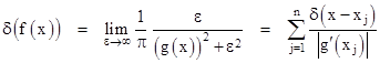
In the limit as ε goes to zero, an expression of this form gives the contribution to the delta function of each root, so we have the relation

Returning to the basic definition of the delta function, we note that it’s possible to define δ(x) in several equivalent ways, including as the limit of certain continuous functions. One particularly useful expression is based on the Cauchy distribution

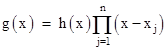
To show explicitly that equation (2) is valid using this simple algebraic definition of δ(x), note that any function g(x) with n distinct real roots x₁ to x_n can be written in the form

where h(x) has no real roots. (See below for comments on the restriction to real roots.) We wish to show that

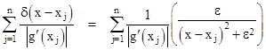
For any given ε we need to show that the summation, with the delta functions written explicitly in the form of (3), equals the original expression with some (possibly re-scaled) value of ε. We have

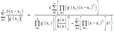
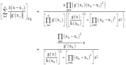
Consolidating the right-hand summation, and neglecting powers of e higher than the first in the numerator, and higher than second in the denominator, we get

Setting x equal to any one of the roots x_k, most of the terms vanish, and we are left with

Noting that

our expression reduces to

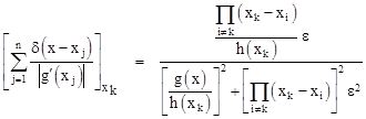
Multiplying through the numerator and denominator by h(x_k)², we arrive at

The right hand expression (multiplied by 1/π) is indeed of the required form, with an epsilon value that is just a constant, g′(x_k), times the epsilon value of the individual delta functions in the summation. This confirms that (2) is valid for the delta function as defined by (3).

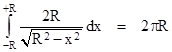
To illustrate the delicacy of the delta functions in applications, consider how we might compute the length of a plane locus by integrating, over the entire plane, the delta function of an expression that vanishes on that locus. For example, one might think that the perimeter of a circle of radius R could be computed as

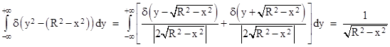
However, taking just the inner integral first, for any constant x in the range –R to +R, we have

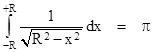
Inserting this back into the double integral (4), and restricting the integration on x to the range –R to +R (which is permissible, since we know the delta function doesn’t vanish outside that range) we get

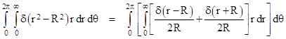
The result is a constant, π, regardless of the radius R, so this clearly does not represent the circumference of the circle. To confirm this result, we might convert to polar coordinates r,θ such that x = r cos(θ) and y = r sin(θ). As described in the note on change of variables in multiple integrals, we have dy dx = r dr dθ, so the double integral (4) becomes

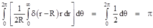
Notice that the argument of the second delta function on the right side is zero only when r equals –R, whereas we are integrating over the range from r = 0 to +R, so that term has no contribution. Thus we have

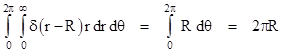
This confirms that the integral is simply π, independent of R, so it does not represent the circumference, even though the argument of the delta function vanishes precisely on the perimeter of the circle. What has gone wrong? The problem is that we took a quadratic function as the argument of the delta function, whereas we ought to take a linear function. For example, in polar coordinates the perimeter of the circle corresponds to the points where r – R vanishes, not where r + R vanishes, so we ought to write

which is indeed the circumference of the circle. Likewise in Cartesian coordinates we should just take the relevant linear condition for the argument of the delta function, and write

Focusing again on just the inner integral for any constant x in the range from –R to R, the argument of the delta function is

which has the derivative

The two roots of g(y) are

so we have

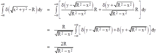
Therefore, making use of equation (2), the inner integral is

Inserting this back into the double integral (5), and again restricting the integration to the range –R to +R as explained previously, we get

as expected. This shows the importance of choosing the right argument for the delta function.

We mentioned previously that the roots of g(x) appearing in equation (2) are real, which is to say, we exclude any roots that are not on the real line. This is because we are integrating on the real numbers, so any roots off the real number line will not be encountered, and hence don’t contribute to the integration. However, we could conceivably apply something like a delta function to integrations over the entire complex plane, in which case the complex roots of the argument would be significant. Of course, we could simply use a product of two ordinary one-dimensional delta functions, one for the real part and one for the imaginary part of the argument, but there might also be a more natural generalization of the delta function to complex numbers.

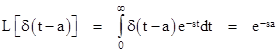
One of the main uses of the delta function arises from its properties when subjected to the common integral transforms.  For example, by definition, the Laplace transform of the delta function is

To show how this is useful, consider an ordinary differential equation

where f(t) = 0 for all t < 0. The driving function f(t) may be of a form that is difficult to handle, but if we replaced f(t) by an impulse function δ(t – t′) occurring at some time t′, we can easily solve the equation using Laplace transforms. Let this solution for an impulse at time t′ be denoted by G(t,t′), so we have

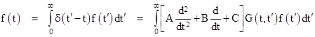
(The function G is a simple example of what is called a Green’s function.) Now, notice that the original driving function can be expressed as

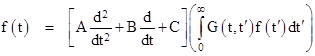
Bringing the differential operator outside the integral, we have

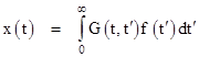
and hence the solution x(t) of the original problem is the second factor on the right side, i.e., the solution can be written in terms of the impulse solution G(t,t′) as

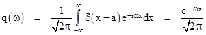
Another reason for the usefulness of Dirac’s delta function is that it has the simple Fourier transform

Applying the inverse Fourier transform, we might think the delta function itself can be expressed as

However, this integral diverges, so this is not a well-defined expression. Nevertheless, if we cut off the integration at large but finite limits, we do get a function that converges on the delta function as the limits increase, so this expression is often presented as a formally valid representation of the delta function.

Incidentally, several features of the delta function discussed above can be seen in Feynman’s 1949 paper on quantum electrodynamics (for which he was later awarded the Nobel prize). His objective is to derive an expression for the amplitude of a particular interaction between two charged particles, corresponding to the Coulomb potential e²/r where e is the electric charge on each particle and r is the distance between the particles. In his notation, the interaction is “turned on” when one particle is at a time and place denoted by event 5, and the other is at the time and place denoted by event 6.  He begins with a double integral over the path parameters dτ₅ and dτ₆ , and to accept contributions only when t₅ = t₆ he multiplies the integrand by the delta function δ(t₅ – t₆), treating the Coulomb interaction non-relativistically as if it acted instantaneously. Thus his expression included a factor of the form

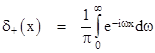
But then he notes that, relativistically, the interaction is not instantaneous, but is retarded by the light-speed delay in propagating from one particle to the other. Thus, is we define the symbols t₅₆ = t₅ – t₆ and r₅₆ = r₅ – r₆, Feynman proposes to modify the formula, substituting in place of δ(t₅₆) the delta function δ(t₅₆ – r₅₆), which signifies that the integral will accept contributions when the particle at 5 is on the forward light cone of the particle at 6. (Note that we are using units such that the speed of light has the value 1.) But now he says “this turns out to be not quite right, for when this interaction is represented by photons, they must be of only positive energy, while the Fourier transform of δ(t₅₆ – r₅₆) contains frequencies of both signs”. He is referring to the representation of the delta function given by equation (6), noting that the integral extends over values of the frequency parameter ω from negative to positive infinity. (Oddly enough, he doesn’t mention that this representation doesn’t actually converge.) To remedy this, he defines a new type of delta function, denoted by δ₊(x), consisting of only the positive frequency parts of the usual delta function, i.e.,

Here the integral ranges from 0 to positive infinite, and we have multiplied by 2 to normalize the result so that the integral of δ₊(x) over all x is 1. Also, Feynman wants to account for the reverse interaction, when the particle at 6 is on the forward light cone of the particle at 5, which happens when t₅₆ + r₅₆ vanishes. He says we need to average the two possibilities, so he replaces (7) with

But recall from our discussion of the composition of functions that

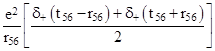
Making use of this fact (which applies to δ₊ as well as to δ), Feynman arrives are the relativistically invariant factor

Without knowing the background for this expression, one might wonder how the amplitude for the Coulomb interaction e²/r can be independent of the distance r₅₆, but we see that the inverse distance is implicit in the delta function of the relativistic squared interval.

Return to MathPages Main Menu