Analysis of Relativistic Orbits

Two quite distinct methods have historically been used to derive the precession rate of relativistic orbits for a test particle moving in the gravitational field of a stationary spherical body of mass m. Both methods begin from the equation (derived from the field equations of general relativity in the note entitled Anomalous Precession)

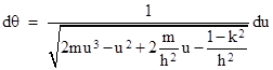
where u = 1/r and h is a constant of motion corresponding to the specific angular momentum of the particle. (Here we are using “geometrical units”, so that the mass m has units of length. For example, the mass of the Sun is 1.475 kilometers.) The first method, used by Einstein in his original 1915 paper, is to simply take the square root of both sides and then evaluate the integral

from one extremum of u(θ) to the next. The clever technique that Einstein used to approximate this elliptic integral is discussed in the note on Conquering the Perihelion. However, there seems no way of applying this technique to give higher orders approximations. Also, this approach yields only an approximation of the angular travel between two successive extremums; it does not give an expression for the actual path of the particle.

The second method that appears frequently in the literature is to actually solve for the orbital path. This is done by first differentiating equation (1) and dividing out the common factors to give the differential equation

At this point it’s helpful to define the dimensionless parameter U = mu. Multiplying through equation (2) by m, and letting σ denote the constant squared ratio (m/h)², we see that it can be written as

Since U = m/r is a small quantity, the term in U² is quite small, so to the first order of approximation this equation is identical to the Newtonian equation

This linear equation has the solution

which describes a simple ellipse with eccentricity ε. This shows that the quantity h²/m is (at least approximately) equal to the semi-latus rectum L of the orbit, so we have σ = (m/h)² ≈ m/L, which is very small for astronomical orbits.

In attempting to solve the non-linear equation (3), one common approach is to substitute the “linear solution” of (4) into the right hand side of (3) to give the linear equation

The solution of the homogeneous equation is the same as before, but now we need a new particular solution to match the new “driving function” on the right hand side. Noting the identities

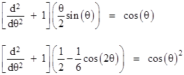
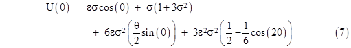
we can easily form a particular solution of equation (6) and combine it with the homogeneous solution to give the (supposedly) improved approximation

As explained at the conclusion of Anomalous Precessions, many text books (including Rindler and d’Inverno) then argue that the third term of this “solution”, containing θsin(θ),  represents the secular advance of the perihelion. Rindler says that, unlike the final term, this term

…cannot be neglected, since it has a resonance factor θ and thus produces a continuously increasing and ultimately noticeable effect.

Likewise d’Inverno says

…the most important correction is the term involving θsin(θ), because after each revolution it gets larger and larger.

Along these same line, Ohanian and Ruffini say that equation (6)

…is mathematically analogous to a harmonic oscillator, with a restoring force –U, two oscillating driving forces proportional to cos(θ) and cos(θ)², and two extra constant forces. The first of the oscillating driving forces is in resonance with the natural oscillations, and therefore it gradually builds up a (relatively) large secular perturbation of the orbit…

Unfortunately, these statements make no sense, because U does not represent the angular position of the test particle, nor of the perihelion of the orbit, it is the inverse of the radial distance of the particle from the gravitating body. A secular change in U on successive orbits would correspond to a secular change in the radius of the orbit, not in the angular position of the perihelion. Actually, since θ is multiplied by sin(θ), the effect of this term would be a progressively increasing amplitude of the radial excursions, meaning that the orbit would be unstable. As explained in a previous note, the argument used by those authors to infer the relativistic precession from equation (7) is self contradictory, since it relies on the “small angle approximation”, which is valid for only a very small portion of a single revolution , which contradicts the claim that the significance of this term is due to it’s cumulative effect over many revolutions.

As explained in the previous note, the real significance of the θsin(θ) term is that it represents the beginnings of a single re-orientation of the orbital axis, as the magnitude of the sine term increases compared with the cosine term. For nearly circular orbits (i.e., with ε much less than 1) this nascent phase shift approximates the precession rate of the actual relativistic orbit, but it is not a resonance effect. Also, the limitation to nearly circular orbits renders this derivation inapplicable to the orbit of the asteroid Icarus (for example), which has an eccentricity of 0.827.

Still, the fact that some expansions of the orbital equation contain terms that, by themselves, represent secular changes in the orbital radius, raises the question of whether the relativistic orbit is strictly stable. Might there be some instability at a sufficiently high order evaluation? To answer this question, we can simply evaluate the power series solution of equation (3). Let the function U(θ) have the power series representation

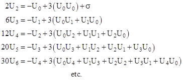
Inserting this into (3) and collecting on powers of θ, we get the conditions

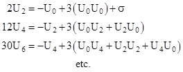
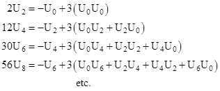
Thus each coefficient is given in terms of a convolution of the previous coefficients. If we choose the origin of θ at any maximum or minimum (aphelion or perihelion), then we have U′(0) = 0 and therefore U₁ = 0. With this condition it follows that U_j = 0 for all odd indices j, because every term in the expressions for such coefficients contains a factor with a lower add index. The conditions for the non-zero coefficients are then

Given the value of the constant coefficient U₀, all the remaining coefficients can be determined, and since only the coefficients with even indices are non-zero, the function U(θ) is even, meaning that it is symmetrical about every maxima and minima. Consequently the path between any maxima and the next minima must be identical, so the orbit is perfectly stable, i.e., the radial excursions have no secular variation, assuming the path contains at least two extremums. (The doesn’t preclude spiral paths, which contain no extremums.)

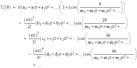
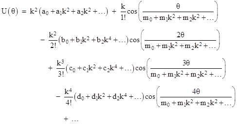
This implies that it must be possible to express U(θ) for a closed orbit purely in terms of cosine functions, with no “secular” functions such as θsin(θ). Of course, this doesn’t mean that expressions for U(θ) cannot include such “secular” terms, but it must be possible to combine all such terms into simple cosine functions. Specifically, the general solution of equation (3) to arbitrary order of approximation can be expressed in the form

where the constant coefficients a_j, b_j, c_j, d_j, … and m_j are functions of ε². The values of these coefficients can be determined simply by substituting this expression into equation (3) written in the form

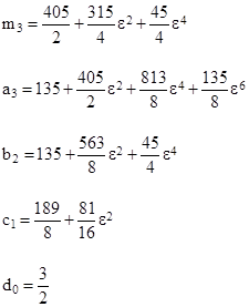
expanding the resulting expression in powers of σ, and then setting the multipliers of each of those powers to zero. In general, those multipliers will be polynomial in cos(θ). To make the multiplier of σ vanish, it is necessary and sufficient to set a₀ = m₀ = 1, which represents the Newtonian approximation, i.e., a simple Keplerian ellipse with no precession. To make the multiplier of σ² vanish, we must set

This level of approximation yields the relativistic precession, which can be seen from the fact that the function repeats itself when the value of θ has gone from 0 to the value that gives 2π as the argument of the cosine, i.e.,

Subtracting 2π from this value of θ gives the precession per revolution, so we have

Since m₀ = 1 and m₁ = 3, this gives to the first order the well known precession 6πσ = 6π(m/h)² per revolution.

To progress to the next level of approximation, we need to make the multiplier of σ³ vanish, which requires us to set

At this level of approximation we find that the rate of precession actually depends (very slightly) on the “eccentricity” of the orbit. Proceeding to the next level, we make the multiplier of σ⁴ vanish by putting

At this level, the left side of (8) differs from zero only by a quantity on the order of σ⁵, which for the planet Mercury’s orbit is roughly 1 part in 10³⁰. This illustrates that any desired degree of approximation can be attained. The formula for U(θ) can also be used to determine the exact shape of the precessing orbit. By setting the denominator of the arguments of the cosine functions to unity, the equations gives the shape when viewed from a “co-precessing” frame. Obviously the orbit is not precisely an ellipse, because of the higher-order terms, so the identification of the constant ε with the “eccentricity” is only an approximate analogy. It is actually just a parameter for the single degree of freedom of the orbits for a given perihelion distance.

We can also determine the equations for null paths, i.e., paths of light rays. For this case the parameter σ equals zero (because h is infinite due to the vanishing of dt along the path), so the equation of motion is

From this we see that the condition on the coefficients of the power series expression are the same as given previously, except that the expression for 2U(θ) does not contain σ. Thus we have

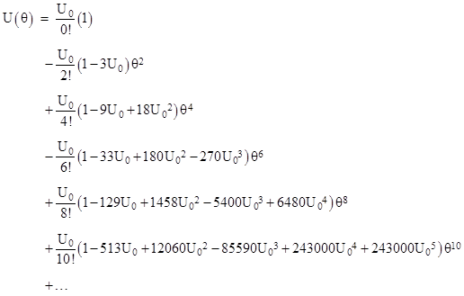
Incidentally, were it not for the factors of n(n–1) on U_n in these recurrence relations, they would generate (with U₀ = 1) the Schröder numbers, as discussed in another note. Expressing all these coefficients in terms of U₀, the function U(θ) can be written as

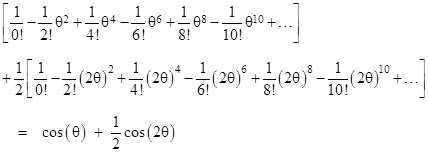
Note that U₀ is approximately m/R where m is the mass of the gravitating body (in geometrical units) and R is the distance of nearest approach. This ratio is many orders of magnitude less than 1 for planetary orbits in the solar system, so we will get reasonably good approximations by considering just terms containing a low power of U₀.  The sum of the first terms of each row gives

which is the approximation corresponding to no deflection at all. For an improved estimate, we add the sum of the second terms, which can be written as

The numbers α₀ = 3/2, α₂ = 3, α₄ = 9, α₆ = 33, etc., can be written explicitly as

so the quantity in the square brackets is

Hence we have the improved approximate solution

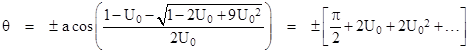
This is already good enough to give the relativistic deflection for a ray of light. The asymptotic directions of the incoming and outgoing rays correspond to the values of θ that make U(θ) vanish, so that the radial distance r goes to infinity. Replacing cos(2θ) with 2cos(θ)² – 1 in the above solution and setting U(θ) = 0 we get the quadratic in cos(θ)

Solving for cos(θ) and taking the inverse-cosine, we get the two asymptotic angles

The difference between these two angles is twice the quantity in the square brackets, so the angle between the incoming and outgoing asymptotes is π + 4U₀.  For a straight line (no deflection) the angle between the asymptotes is simply p, so the excess angle, representing the deflection of the light ray, is 4U₀.  As noted above, the coefficient U₀ corresponds to m/R, where m is the mass of the gravitating body (in geometrical units) and R is the perigee distance, so the light deflection can be written as d = 4m/R.

However, as in the case of bound timelike orbits, extending this analysis to higher orders of approximation is not straightforward. The next sequence of coefficients from the power series expansion of U(θ) is 18, 180, 1458, 12060, 103698, 913140, etc., which isn’t easily expressed in closed form as a sum of powers of 1, 4, 9, etc.  We might think it would be possible to simply set σ = 0 in the solution derived for timelike orbits, but this would require setting ε to infinity (so that σε has some finite value), which then results in some higher order terms going to infinity. Another approach would be to iteratively substitute solutions of the homogeneous equation into the right hand side of (9) to give progressively more accurate forcing functions. This leads to terms with factors such as θsin(θ), but it ought to be possible to express the solution entirely in terms of cosines. To do this, we again allow for “precession” of the angular variable, and posit a solution of the form

Now, by the same method as described for timelike paths, we can insert this into the lightlike equation of motion (9) and determine the required values of the coefficients. This yields the results

When expressed in this form, the path of light has a “precession” component, just as do the closed timelike orbits, although the effect of this precession is negligibly small for hyperbolic orbits, at least in the weak field regime.

Return to MathPages Main Menu