Eigen Systems

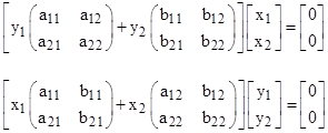
A previous note described the duality between eigenvalues and eigenvectors. Here we describe some examples in more detail, and consider possible applications to quantum mechanics. Consider first the two equivalent systems of equations shown below

Conventionally we would multiply through each of these equations by the inverse of one of the two matrices, and then for the first form we would regard the ratio y₁/y₂ as the eigenvalue, and the quantities x₁ and x₂ as the components of the eigenvector. However, the second form shows that we can just as well regard the ratio x₁/x₂ as the eigenvalue, and the quantities y₁ and y₂ as the eigenvector. Thus the distinction between eigenvalues and eigenvectors is artificial, and becomes even less meaningful when we consider systems with more than two dimensions. So we will simply refer to both x and y as vectors.

The matrices in the two forms are related in a simple and reciprocal way: The kth matrix of each form consists of the kth columns of the matrices of the other form. For example, in the system above, the first matrix of the second form consists of the first columns of the matrices of the first form, and the second matrix of the second form consists of the second columns of the matrices of the first form. This mapping applies (for “square” systems) to systems of any number of dimensions.

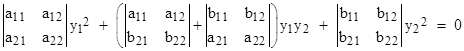
We know the determinants of the combined matrix (in square brackets) on the left sides of the two equations above must vanish. The first of these leads to the following quadratic equation on the components of y:

Setting the determinant of the matrix on the left side of the second form leads to a similar quadratic equation in the components of x, after making the column transpositions noted above. To give a concrete example, consider a system defined by the matrices:

For this system the vanishing of the determinants of the two forms gives the quadratics

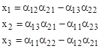
Solving these for the ratios y1/y2 and x1/x2, and then using the original system to establish the correspondence between these solutions, we get the two results

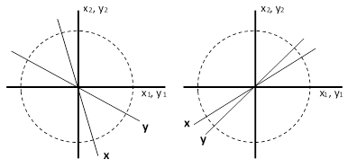
where the ± signs are either both plus or both minus. Viewing x and y as vectors, the two solutions can be depicted as shown below.

The overall space essentially consists of the one-dimensional bi-podal circle (identifying opposite points of the circle), and these figures illustrate how the system equations constrain the vectors to be in one of two sets of corresponding subspaces (which are single points in this simple example).

With a three-dimensional system of equations the overall space can be represented by the two-dimensional surface of a sphere, again identifying opposite points, and the system equations constrain the vectors to one of three sets of corresponding subspaces, although in this case the sub-spaces are loci rather than single points. The two equivalent forms of the system equations are

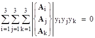
where A₁, A₂, and A₃ are 3x3 matrices, and the hatted symbols signify that the columns have been subjected to the transformation explained above (i.e., the kth matrix of each form consists of the kth columns of the matrices of the other form). As before, we set the determinants of the coefficient matrices (in square brackets) to zero, to give conditions on the x and y vectors. In this case we get cubic equations in the three components. The cubic equation for the y components can be written as

where the symbol in curly braces signifies the matrix with the first row taken from A_i, the second row taken from A_j, and the third row taken from A_k. The cubic in the components of x has the same form, with the hatted matrices replacing the unhatted matrices.

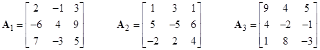
As an example, consider the system defined by the following three matrices

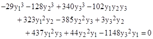
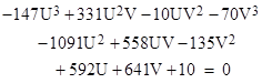
For this system the components of y must satisfy the homogeneous cubic

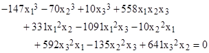
and the components of x must satisfy the homogeneous cubic

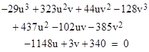
Dividing through the “y” equation by y₃³, and letting u = y₁/y₃ and v = y₂/y₃, we have a cubic in two variables

Likewise if we divide through the “x” equation by x₃, and let U = x₁/x₃ and V = x₂/x₃, we have the cubic in two variables

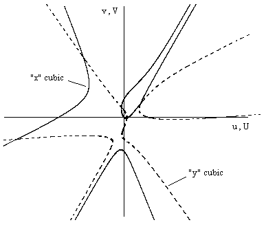
The loci of real values that satisfy these cubics are shown in the plot below.

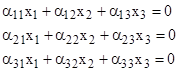
Both of the loci in this case consist of 3 separate branches. Given any value of the y vector on its solution locus, the corresponding x vector on its locus is uniquely determined, and vice versa. This follows because, given values of y₁, y₂, y₃, for which the determinant of the system equation vanishes, we have equations for x of the form

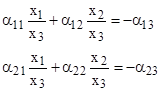
where the α_j are functions of y, and we can divide through any two of these equations, say, the first two, by x₃, to give

from which we get, up to arbitrary scale factor, the x components

We can normalize both the x and y vectors to unit vectors, represented by points on a sphere, with the understanding that opposite points on the sphere are identified with each other (since only the axial directions in this space are significant).

Recalling that conventional quantum mechanics can be expressed in terms of matrices (as in the original formulation of Heisenberg, Born, and Jordan), it would be interesting to know whether generalized eigensystems discussed here could be used to represent some generalization of quantum mechanics. In the usual matrix formulation, a dynamical variable is represented by a Hermitian matrix Q (usually of infinite size), and a measurement of that variable associated with a given physical system is characterized by the eigenvalue relation Qx = λx where the real-valued scalar λ is the result of the measurement and the column vector x is the state of the physical system immediately following the measurement. According to our generalization we would regard λ as the ratio -y₁/y₂ of the components of the “y” vector representing part of the state vector of the measuring system, and we would regard Q as the ratio Q₁/Q₂ of two matrices, so the measurement condition can be written as

By increasing the dimension of the y vector, we are essentially increasing the number of “measured variables”, and hence we must increase the number of matrices. For example, the equation

might be regarded as representing a measurement of two variables, λ₁ = y₁/y₃ and λ₂ = y₂/y₃, with the corresponding matrices Q₁/Q₃ and Q₂/Q₃ representing those two dynamical variables. In this context we would expect the ratios of the y values to be real while the ratios of the components of x may be complex. Also, as noted above, the dimensions of Q and x are generally infinite while we have only a finite number of y values. We would have to imagine a system with an infinite number of observables, and allow complex eigenvalues, to make the system fully symmetrical.

As would be expected for the simultaneous “measurement” of multiple variables, the result is under-specified, as indicated by the loci of solutions (which we might call the eigen spaces). A measurement of a single variable is a special kind of interaction contrived to be just two-dimensional in one of the vectors, so that the systems is resolved uniquely into one of a countable number of individual eigenstates, but more general interactions, not designed as “measurements”, yield a less definite state reduction. Instead, such interactions merely send the system to one of a countable number of sub-spaces (the eigen spaces). It’s difficult to see how a finite set of individual basis vectors could be chosen, so it might be necessary to generalize this to a set of “basis spaces”.

Return to MathPages Main Menu