The Dirac Equation

Quantum mechanics is based on a correspondence principle that maps classical dynamical variables to differential operators. From the classical equation of motion for a given object, expressed in terms of energy E and momentum p, the corresponding wave equation of quantum mechanics is given by making the replacements

and then treating the resulting expression as a differential operator on the wave function of the object. For example, recall that the non-relativistic momentum components of a particle are p_x = mv_x, etc., and the kinetic energy is m|v|²/2 = |p|²/(2m), so the equation of motion for a free particle (i.e., no potential energy) is

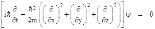
where E is the total energy. Making the replacements noted above, and applying the resulting operators to the wave function ψ of the particle, this gives

which is the non-relativistic Schrödinger equation of a free particle of mass m. This equation is valid only if the speed of the particle is small compared with the speed of light, because it was based on the non-relativistic expression (1) for the energy. To cover relativistic speeds we must use the relativistic relation between energy and momentum, which is E² = m² + |p|². Thus we have

If we were to replace E in this equation with the operator ih(∂/∂t), the resulting equation of motion would involve the second time derivative of the wave function, in contrast with the non-relativistic Schrödinger equation, in which only the first time derivative of the wave function appears. In his book “The Principles of Quantum Mechanics” Dirac wrote that “we deduced from quite general arguments that the wave equation must be linear in the operator ∂/∂t”, and that an equation of motion involving the second time derivative would not be “of the form required by the general laws of the quantum theory”. The detailed justification of this statement involved the need for the probability density of the wave to be always positive. In later years Dirac described his motivations differently, explaining that he hadn’t pursued the quadratic form (leading to what is now called the Klein-Gordon equation) because it seemed inconsistent with his work on “transformation theory” based on the first-order time derivative.

I think [the transformation theory] is the piece of work which has most pleased me of all the works I’ve done in my life… [it] had become my darling. I was not interested in considering any theory which would not fit in with my darling. Therefore, the linearity of  ∂/∂t was absolutely essential to me; I just couldn’t face giving up the transformation theory.

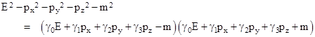
Whatever the motivation, Dirac sought a wave equation whose solutions would be solutions of (2), but that was linear in E. His approach was to hypothesize that (2) can be expressed as the product of “conjugate” linear factor. Specifically, he postulated a set of basis variables γ₀, γ₁, γ₂, and γ₃ (not necessarily commuting) such that

Expanding the product and collecting terms, we find that this is a valid equality if and only if the four variables γ_j satisfy the relations

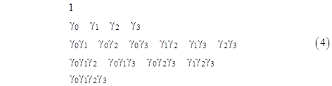
for all i,j = 0,1,2,3 with i ≠ j. These four quantities, along with unity, form the basis of what is called a Clifford algebra, after William Clifford, who investigated such mathematical structures in the late 1800s. (Dirac was unaware of this history.) It’s easy to see that any product of two or more of these entities can be reduced to a unique signed product of zero, one, two, three, or all four of the them with indices in increasing order. For example, we have the identity

which is found by repeated transpositions of neighboring entities in the left hand string, reversing the sign with each transposition, and consolidating squared entities using the idempotence relations noted above. Thus every product of two or more of the four entities is equivalent to one of the 16 signed expressions

These may be regarded as the “units” of this algebraic structure, similar to the two signed units 1 and i of ordinary complex numbers. Obviously each of these 16 expressions, when squared, reduces to either +1 or –1. Within this algebraic structure the quadratic relativistic equation relating energy, momentum, and mass can be factored as noted above, and the full equation will be satisfied if either of the factors vanishes. Focusing on the factor with positive mass, this gives the condition

Making the usual quantization substitutions for E and p, dividing through by i and h-bar, and applying the resulting expression as an operator on a wave function ψ, Dirac arrived at the equation

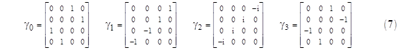
for a free particle of mass m. We might be content at this point, having found a wave equation with coefficients involving some non-real basis variables, just as the original Schrödinger equation involves the imaginary variable i. However, unlike the ordinary complex numbers, the multiplication of these new basis variables γ_j is not commutative, a fact which suggests some underlying structure. (The articulation of non-commuting entities into structures of commuting entities is a useful heuristic principle, although it is rarely mentioned explicitly.) Accordingly, Dirac sought a representation of these basis variables in terms of complex numbers. He found that the γ_j variables can be represented by 4x4 matrices with complex elements, with the understanding that the symbols “1” and “0” in equation (6) represent the identity matrix and the null matrix respectively. For example, the following matrices satisfy all the requirements:

These can be used to generate the 16 “units” given by (4), and then every 4x4 matrix with complex elements can be expressed as a linear combination of those 16 matrices. Since the operator is now a 4x4 matrix, the wave equation (6) is a matrix equation, which implies that the wave function of this particle must actually have four components, so it can be expressed as the vector

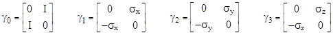
Thus, in a sense, we must consider four distinct versions of the particle. However, the elements of the γ matrices are not independent, as shown by the fact that the γ matrices listed above can be written in the form

where I is the 2x2 identity matrix and σ_x, σ_y, σ_z are the 2x2 Pauli spin matrices

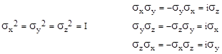
These are called “spin” matrices because they are characterized by the relations

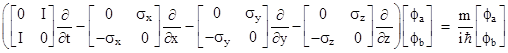
which are analogous to the relations for the components of angular momentum of a classical particle. Expressing the vector of wave functions as a two-dimensional vector of two-dimensional vectors ϕ_a and ϕ_b by

we can write Dirac’s wave equation explicitly as

Carrying out the matrix multiplications, this represents the following two equations

As a check, by substituting the expression for ϕ_b from the second equation into the first, and simplifying by making use of the properties of the spin matrices, we can verify that the two-dimensional vector ϕ_a satisfies the Klein-Gordon equation

which we recall is simply the quantized version of the relativistic energy-momentum equation E² – p² = m². Likewise we can show that the two dimensional vector ϕ_b satisfies the very same equation, and therefore (as required) each of the four components ψ₁, ψ₂, ψ₃, ψ₄ of the original four-dimensional vector of wave functions individually satisfies the Klein-Gordon equation. (Equations (8) and (9) can be seen as a generalization of the Cauchy-Riemann conditions for analyticity, with ϕ_a and ϕ_b being analogous to conjugate harmonic functions.) However, these equations also show that the four components of ψ are not independent, because given any solution ϕ_a of (10) we can compute ϕ_b using (9). These wave functions will then automatically satisfy (8) as well. Therefore, either ϕ_a by itself or ϕ_b by itself is sufficient to determine the complete wave function ψ for a given basis. Also, comparing equations (8) and (9), we see that ϕ_a and ϕ_b are symmetrical except that the signs of the Pauli spin matrices are reversed. Thus a particle described by Dirac’s equation has just two possible intrinsic states relative to a given basis, corresponding to the left-handed and right-handed spin states of the particle for that basis.

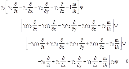
One useful way of expressing the wave function of such a particle is as a linear combination of two mutually exclusive (i.e., “orthogonal”) components. Notice that, of the 16 “unit” matrices identified in (3), only the matrix given by γ₀γ₁γ₂γ₃ anti-commutes with all four of the generators. For convenience we will give this special unit matrix, multiplied by i (which of course doesn’t affect the anti-commutative properties), the special name γ₅, which is to say, we define

The factor of i is included so that γ₅² = I, which will prove to be convenient below. Since this matrix anti-commutes with each of the generators, it follows that multiplying through equation (6) by γ₅ gives

Therefore, if ψ is a solution of Dirac’s equation (6), it follows that γ₅ψ is also a solution, but with the momentum and the energy negated relative to the sign of the mass. Alternatively we can say that  γ₅ψ is a solution of the “negative mass” version of Dirac’s equation, i.e.,

Recall that this corresponds to the other factor of the equation E² – p² – m² = 0, so solutions of this equation are, strictly speaking, equally valid solutions of the Klein-Gordon equation from which we began. Of course if m = 0 there is no distinction between the two factors. Even for cases when m is not zero, the distinction between the two factors may be extremely small if the energy and momentum are extremely large, i.e., for a particle moving at close to the speed of light.

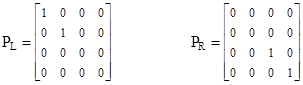
Now, since for any given solution ψ, the wave functions Iψ and γ₅ψ are also solutions, and since the Dirac equation is linear, any linear combination of solutions is also a solution. Therefore, if we define the matrices P_L = (I – γ₅)/2 and P_R = (I + γ₅)/2, we know that P_Lψ and P_Rψ are both solutions, which we will call ψ_L and ψ_R respectively. Remembering that  γ₅² = I, it’s easy to show that the P_L and P_R matrices have the following properties

so they can be regarded as a complete set of projection operators. Furthermore, based on the generators (7), the matrix γ₅ is diagonal, and we have

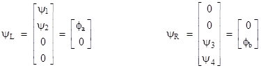
Therefore these projection operators resolve the full wave function for a given particle into two parts, namely ψ = ψ_L + ψ_R, where the non-zero parts of ψ_L and ψ_R are just the two-dimensional vectors ϕ_a and ϕ_b discussed previously, i.e.,

As explained previously, ϕ_a and ϕ_b are the same except for having opposite intrinsic spin. The fact that particles satisfying the Dirac equation (such as electrons) have two distinct states of quantum spin is highly consequential, because it accounts for the valency properties of atoms (each quantum “orbit” can be occupied by two electrons with opposite spins), which makes possible the whole variety of chemical interactions in nature.

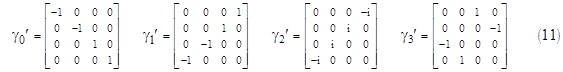
This set of γ matrices discussed above is not unique. For example, if we replace the original matrix γ₀ in (7) with the matrix γ₅, we get the equally satisfactory set of generators

This basis is convenient for dealing with stationary or slow-moving particles. To see why, notice that the analogs of equations (8) and (9) for this basis are

where ϕ_a and ϕ_b are the two-dimensional vector functions discussed previously. Now, for a stationary particle, the wave function ψ should be independent of time, except for possibly an unobservable phase advance, which is to say, the wave function can be factored into a spatial part and a unit complex temporal part as follows

for some real constant ω, where f is a four-dimensional vector of spatial functions. Thus we can write

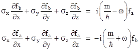
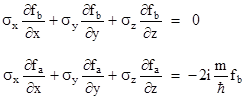
where f_a and f_b are two-dimensional spatial wave functions. Substituting for these vectors in equations (12) and re-arranging terms, we get

It follows that f_a and f_b must each satisfy a relation of the form

Thus in order for f_a and f_b to be harmonic functions, the quantity in parentheses in this equation must vanish, so choosing the positive frequency solution, and noting that (since the particle in this case is assumed to be stationary or nearly so) we have E = m, we find that the phase angular speed w for a stationary particle must be related to the mass-energy by

With this condition the preceding equations then reduce to

We expect both of these “spin divergences” to vanish, so the second equation requires us to set f_b = 0. Hence, with this basis applied to stationary (or approximately to slowly moving) particles, we have ϕ_b = 0 and

An abbreviated version of this approach is to note that, for a stationary particle (i.e., with zero momentum), equation (5) reduces to γ₀’E – Im = 0. (Note that we are using the primed γ basis.) Making the usual quantum substitution for E, the corresponding Dirac equation is simply

As before, we express the wave function of a stationary particle in the form (13). Making this substitution into the above equation and simplifying, we get

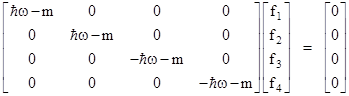
Inserting the γ₀’ matrix and writing this equation explicitly, we have

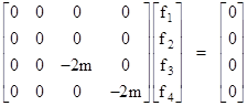
This shows that if ω is not equal to  then f must be identically zero. The only non-vanishing solution is with ω equal to . Assuming a positive frequency, the preceding equation becomes

Therefore, we find (again) that ϕ_b must vanish, and ϕ_a is of the form

The two components of ϕ_a (i.e., ϕ₁ and ϕ₂) consist of the two spin states of the particle.

In the preceding discussion we’ve mentioned two different sets of γ matrices, defined in (7) and (11), that each represent a satisfactory basis for evaluating Dirac’s equation. These are called the Weyl basis and the Dirac basis respectively. As noted above, the Weyl basis is convenient for high-speed electrons (for which the momentum is much larger than the rest mass), and the Dirac basis is convenient for stationary or low-speed particles.

However, these are by no means the only two satisfactory sets of basis matrices. In fact, it’s easy to verify that if γ_i, i = 0,1,2,3 is a set of matrices that satisfy all the requirements of Dirac’s equation, then for any invertible 4x4 matrix μ the matrices given by μγ_jμ^–1 for j = 0,1,2,3 also satisfy all the requirements. This is vitally important for achieving one of Dirac’s main objectives, which was to find a Lorentz invariant wave equation for a particle. It isn’t obvious that a linear equation of the kind sought by Dirac (as opposed to, say, the Klein-Gordon equation) could ever be relativistic, but remarkably it turns out that Dirac’s equations actually is invariant under Lorentz transformations, provided we take into account the transformation properties of the γ matrices.

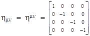
To simplify the notation, let x⁰, x¹, x², x³ denote the coordinates t, x, y, z respectively (where the superscripts are indices, not exponents). Also, let the contravariant and covariant components of a given 4-vector be denoted with super-scripted and sub-scripted indices respectively, and let the fundamental metric tensor of (flat) spacetime be denoted by

Recall that the contravariant and covariant components of any 4-vector “a” are related by

where now we adopt the convention that summation over any repeated index in a given term is implied. The Lorentz-invariant scalar product of two 4-vectors “a” and “b” is then expressed as

The differential operators ∂/∂x^μ transform as the components of a covariant 4-vector, so for convenience we will denote them by ∂_μ , and using the summation convention we can re-write the Dirac equation (6) as

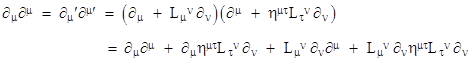
Of course, the γ matrices are not 4-vectors, so the first term inside the parentheses of this equation is not a scalar, it is the sum of four matrices, each multiplied by one of the ∂_μ scalar components. Our use of superscripts here instead of subscripts for the γ matrices is just for typographical consistency. An infinitesimal Lorentz transformation of the column vector ∂_μ can be written (up to the first order) as

where L is a 4x4 matrix whose elements are infinitesimal quantities of the first order. Note that the components of L are anti-symmetric, which follows directly from the fact that the scalar product is invariant, i.e., we have

To the first order this reduces to

so we have L^μν + L^νμ = 0.

Solving the four linear equations (15) for the ∂_μ , and again omitting second order terms in the infinitesimal matrix L, gives the reciprocal relation

Substituting into (14) gives

By simply changing the order of summation of the first term, we have the identity

so equation (16) can be written as

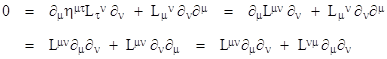
Now suppose we define another 4x4 matrix, which we will call M, whose elements (like those of L) are infinitesimal quantities of the first order, and are such that

for μ = 0,1,2,3. These four equations uniquely determine the matrix M (as will be shown below). If we now multiply through equation (17) on the left by the matrix I+M we get

Expanding the coefficient of ∂_μʹ in this expression gives

The last term contains a product of M and L, each of which is infinitesimal to the first order, so it is second order and can be dropped. We can also replace the third term by making use of (18), so we have

Substituting back into equation (19), and noting that each ∂_μʹ is a scalar so it commutes with (I+M), we can factor (I+M) on the right side, to give

Therefore, if we define

we have

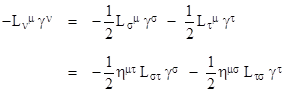
which is of the same form as the original Dirac equation. Of course, before we can assert that this equation is invariant under Lorentz transformations, we need to show that ψʹ(x’) represents the same physical wave function with respect to the spacetime coordinates x’ as is represented by ψ(x) with respect to the spacetime coordinates x. This requires us to show that they have the same probability density at any given event. First we need to determine an explicit expression for the matrix M in terms of the infinitesimal Lorentz transformation L. Recall that we defined M implicitly by the equation (18)

The right hand side can be split into two parts

Making use of the anti-symmetry of L, this can be written as

Noting that equations (3) can be summarized by the expression

we can substitute for η in the preceding equation to give

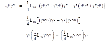
Therefore, equation (18) implies that

Again it must be kept in mind that the γ^μ symbols represent matrices, not vectors as their single suffixes might suggest, so M is a matrix, not a scalar.

Now, to prove that the wave function in (22) represents the same physical situation as the original wave function, recall that in non-relativistic quantum mechanics the probability density is considered to be invariant, given by multiplying the state vector by its conjugate transpose, but in a relativistic theory the probability density cannot be invariant under Lorentz transformations if probability is to be invariant, just as the charge density cannot be invariant if charge is invariant. Instead, the probability density as a function of space and time must transform like the time component of a 4-vector (just as does charge density). To determine the entire 4-vector representing both the probability density and the probability current, recall that, as discussed previously, the four components of ψ can be split into two inter-related bi-vectors ψ_a and ψ_b, and the interchange of these two represents another kind of “transposition” (along with transposing the overall vector and taking the complex conjugates of the components). Hence, although the probability density of an ordinary state vector is generally of the form

we might expect this to be just one component of a complete expression involving the transposition of the two bi-vectors in the leading factor, which gives

Notice that the matrix transposing the two bi-vectors is the same as γ⁰, so we are led to hypothesize that instead of considering just the expression  we should consider . In effect, the leading factor is subjected to three transformations, consisting of the overall transposition, the complex conjugation of the elements, and the transposition of the two bi-vectors. The four components of our probability density-current vector are then hypothesized to be

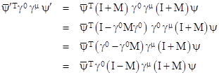
To investigate whether this gives a logically self-consistent theory, recall that the transposed complex conjugate of our transformed state vector ψʹ in terms of ψ can be found from equation (21), noting that the transpose of a product is the product of the transposes in reverse order. Thus we have

Now, the matrix M is not anti-Hermitian, so we can’t simply write the second factor on the right side as (I – M). However, it’s easy to verify that each term of M is made anti-Hermitian by multiplying it on both sides by γ⁰. Consequently we have

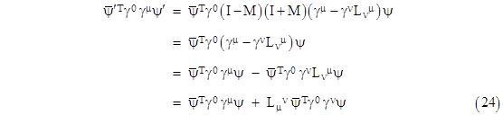
Making use of this relation, and neglecting second-order terms in the infinitesimal matrix M, we can evaluate the four scalar quantities given by

Substituting from (20) this becomes

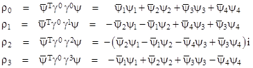
where, in the last step, we’ve made use of the fact that an infinitesimal Lorentz transformation L is anti-symmetric. Thus the four scalar quantities defined by the above equation transform as the components of a 4-vector, with the components (relative to this basis) given by

The “time” component r₀ of this 4-vector reduces to . This positive-definite quantity represents the probability density, which transforms (as it should) under a Lorentz transformation in the same way as the time coordinate of a timelike interval. Thus Dirac achieved his objective of finding a relativistic and positive-definite probability density for the electron. The “space” components ρ₁, ρ₂, ρ₃ represent the probability current, i.e., the probability of the particle crossing a given plane (normal to a given direction) per unit area and per unit time. The invariant squared magnitude of the density-current is

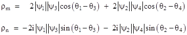
If we express each of the four components of the wave function in the form

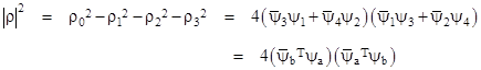
then the squared magnitude of the density-current (in this basis) can be written as

This is obviously real-valued, and it is positive definite, because the minimum value it can take is with the cosine equal to –1, in which case the quantity factors as the square of a real number.

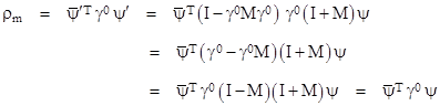
Another invariant quantity is given by

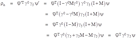
where, as always, we omit second-order terms in the infinitesimal M. Also, since γ₅ anti-commutes with each of the γ^μ, it follows that γ₅ commutes with M, and therefore we have still another invariant, given by

These last two invariants can be regarded as orthogonal components of the density-current vector, since their magnitudes are given by

and hence the invariant magnitudes are related to the magnitude of the density-current by

Regarding the above derivations, it’s worth noting that Dirac originally chose a basis in which the coefficient of ∂₀ was the identity matrix I, and the coefficient of m, which he called γ_m, was not equal to I. This is in contrast to our discussion above, where we’ve done just the opposite, i.e., we’ve chosen a basis in which the coefficient of m is the identity matrix, and γ⁰ is not. In Dirac’s basis, since γ⁰ = I, the matrix M itself is anti-Hermitian, which simplifies some of the results, but is less consistent with modern usage.

As discussed previously, the four components of the wave function ψ can be split into two sets, ψ_a and ψ_b, each consisting of two components, and these two sets are redundant, so the particle can be represented by just two wave functions, corresponding to the two possible spin states for a given basis. However, in another sense, the fact that the full wave function has four components instead of just two is very significant, because the transformation from one basis to another can make use of these four degrees of freedom to produce an unexpected (in 1927) consequence. Recall that the matrices denoted by γ_i, i = 0,1,2,3 together with the identity matrix generate a group of 16 signed “unit” matrices, and this same group can be generated by some other subsets. For example, the group of units (4) can be generated by the four matrices

Since the four γ matrices satisfy all the required conditions, they represent an equally valid basis for Dirac’s equation (6), which can therefore be written in the form

Notice that γ₂ is the only one of the original γ matrices that is imaginary, and it appears as a factor in each of the γʹ matrices, so all of the γʹ matrices are imaginary. Now, if we apply complex conjugation to every quantity appearing in an equality, replacing each i with –i, the equality still holds. Noting that every term in (26) has a factor of i, it follows that the complex conjugate of ψ is also a solution of (26). For an electron, this complex conjugate solution represents the “positron”, i.e., the anti-particle of the electron. If the interaction with an electromagnetic field is included in the Dirac equation, the charge of the particle is negated for the conjugate solution, so the positron has positive electric charge, but the same mass and spin attributes as an electron.

Incidentally, Dirac originally thought his equation applied to every particle of mass m, and hence that all massive particles must have “spin 1/2”. This is indeed the case for the particles that were known in 1928, namely electrons, protons, and neutrons, but other kinds of particles (including photons) are known to have spins different from h-bar/2. Dirac’s explanation for this is interesting:

The answer is to be found in a hidden assumption in our work. Our argument is valid only provided the position of the particle is an observable. If this assumption holds, the particle must have a spin angular momentum of half a quantum. For those particles that have a different spin the assumption must be false and any dynamical variables x₁, x₂, x₃ that may be introduced to describe the position of the particle cannot be observables in accordance with our general theory. For such particles there is no true Schrödinger representation. One might be able to introduce a quasi wave function involving the dynamical variables x₁, x₂, x₃, but it would not have the correct physical interpretation of a wave function—that the square of its modulus gives the probability density. For such particles there is still a momentum representation, which is sufficient for practical purposes.

Dirac’s theory of the electron was remarkably successful, especially in its prediction of the positron, which was discovered experimentally just two years after Dirac published his prediction. However, to account for the fact that matter doesn’t degenerate into negative-energy states, Dirac found it necessary to propose a “sea” of anti-particles, and then invoke the Pauli exclusion principle, arguing that all the negative energy states were occupied. The positron was then conceived as a “hole” in the Dirac sea. In retrospect, this “hole” explanation seems unconvincing, because we now know that all particles, not just fermions for which the Pauli exclusion principle applies, are accompanied by anti-particles, so the “hole” interpretation doesn’t work. Weinberg asked Dirac about this in 1972, and Dirac replied that he didn’t regard massive bosons as “important”. It isn’t clear what he meant by this (perhaps he meant that such particles are not elementary?), although Weinberg notes that a few years later Dirac acknowledged that “for bosons we no longer have the picture of a vacuum with negative energy states filled up… the whole theory becomes more complicated”, presumably referring to the creation and annihilation operators of modern quantum field theory. The modern view seems to be that Dirac’s prediction of the positron was not entirely well-founded, although it certainly does emerge rather unavoidably from consideration of the two roots of E² – |p|²= m².

The most profound implication of Dirac’s equation was that any relativistic description of a particle necessarily involves not just the wave function of a single particle, but multiple wave functions representing the potential for other particles. The first quantization in physics gave a field representation for all the possible states of a given particle, by treating the observable properties (such as position and momentum) as operators on a wave function. The “second quantization”, suggested by Dirac’s equation, then consists of treating this quantum wave function itself as an operator, giving a field representation of all the possible quantum fields. We might says that second quantization considers “the field of all fields”. It’s remarkable that general relativity (the other fundamental theory of physics developed in the early 20th century) also involves a consideration of the field of all fields, albeit in a completely different sense. In both cases this leads to non-linearities, and in both cases the theories are found to entail infinities – if we regard them as exact to all orders, rather than just low-energy “effective” field theories.

Return to MathPages Main Menu