Bras, Kets, and Matrices

When quantum mechanics was originally developed (1925) the simple rules of matrix arithmetic was not yet part of every technically educated person’s basic knowledge. As a result, Heisenberg didn’t realize that the (to him) mysterious non-commutative multiplication he had discovered for his quantum mechanical variables was nothing other than matrix multiplication. Likewise when Dirac developed his own distinctive approach to quantum mechanics (see his book “The Principles of Quantum Mechanics”, first published in 1930) he expressed the quantum mechanical equations in terms of his own customized notation – which remains in widespread use today – rather than availing himself of the terminology of matrix algebra. To some extent this was (and is) justified by the convenience of Dirac’s notation, but modern readers who are already acquainted with the elementary arithmetic of matrices may find it easier to read Dirac (and the rest of the literature on quantum mechanics) if they are aware of the correspondence between Dirac’s notation and the standard language of matrices

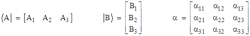
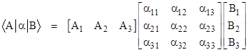
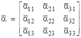
The entities that Dirac called “kets” and “bras” are simply column vectors and row vectors, respectively, and the linear operators of Dirac are simply square matrices. Of course, the elements of these vectors and matrices are generally complex numbers. For convenience we will express ourselves in terms of vectors and matrices of size 3, but they may be of any size, and in fact they are usually of infinite size (and can even be generalized to continuous analogs). In summary, when Dirac refers to a “bra”, which he denoted as <A|, a “ket”, which he denoted as |B>, and a measurement operator α, we can associate these with vectors and matrices as follows

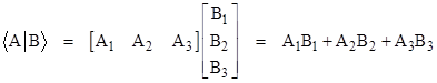
The product of a bra and a ket, denoted by Dirac as <A||B> or, more commonly by omitting one of the middle lines, as <A|B>, is simply the ordinary (complex) number given by multiplying a row vector and a column vector in the usual way, i.e.,

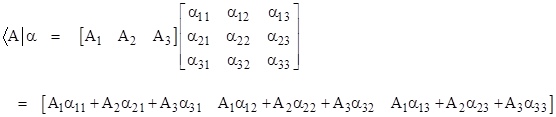
Likewise the product of a bra times a linear operator corresponds to the product of a row vector times a square matrix, which is again a row vector (i.e., a “bra”) as follows

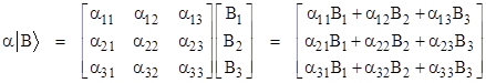
and the product of a linear operator times a ket corresponds to the product of a square matrix times a column vector, yielding another column vector (i.e., a ket) as follows

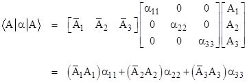
Obviously we can form an ordinary (complex) number by taking the compound product of a bra, a linear operator, and a ket, which corresponds to forming the product of a row vector times a square matrix times a column vector

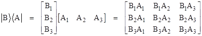
We can also form the product of a ket times a bra, which gives a linear operator (i.e., a square matrix), as shown below.

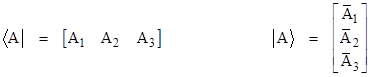
Dirac placed the bras and the kets into a one-to-one correspondence with each other by defining, for any given ket |A>, the bra <A|, which he called the conjugate imaginary. In the language of matrices these two vectors are related to each other by simply taking the transpose and then taking the complex conjugate of each element (i.e., negating the sign of the imaginary component of each element). Thus the following two vectors correspond to what Dirac called conjugate imaginaries of each other.

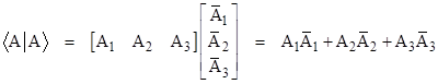
where the overbar signifies complex conjugation. Dirac chose not to call these two vectors the complex conjugates of each other because they are entities of different types, and cannot be added together to give a purely real entity. Nevertheless, like ordinary complex numbers, the product of a bra and its (imaginary) conjugate ket is a purely real number, given by the “dot product”

The conjugation of linear operators is formally the same, i.e., we take the transpose of the matrix and then replace each element with its complex conjugate. Thus the conjugate transpose of the operator α (defined above) corresponds to the matrix

This is called the adjoint of α, which we denote by an overbar. Recall that the ordinary transpose operation satisfies the identity

for any two matrices α and β. It’s easy to verify that the conjugate transpose satisfies an identity of the same form, i.e.,

The rule for forming the conjugate transpose of a product by taking the conjugate transpose of each factor and reversing the order is quite general. It applies to any number of factors, and the factors need not be square, and may even be ordinary numbers (with the understanding that the conjugate transpose of a complex number is simply its conjugate). For example, given any four matrices α,β,γ,δ with suitable dimensions so that they can be multiplied together in the indicated sequence, we have

This applies to the row and column vectors corresponding to Dirac’s bras and kets, as well as to scalar (complex) numbers and square matrices. One minor shortcoming of Dirac’s notation is that it provides no symbolic way of denoting the conjugate transpose of a bra or ket. Dirac reserved the overbar notation for what he called the conjugate complex, whereas he referred to the conjugate transpose of bras and kets as conjugate imaginaries. Thus the conjugate imaginary of <A| is simply written as |A>, but there is no symbolic way of denoting ‘the conjugate imaginary of <A|α’, for example, other than explicitly as .

We might be tempted to define the “real part” of a matrix as the matrix consisting of just the real parts of the individual elements, but Dirac pointed out that it’s more natural (and useful) to carry over from ordinary complex numbers the property that an entity is “real” if it equals its “conjugate”. Our definition of “conjugation” for matrices involves taking the transpose as well as conjugating the individual elements, so we need our generalized definition of “real” to take this into account. To do this, we define a matrix to be “real” if it equals its adjoint. Such matrices are also called self-adjoint. Clearly the real elements of a self-adjoint matrix must be symmetrical, and the imaginary parts of its elements must be anti-symmetrical. On the other hand, the real components of the elements of a purely “imaginary” matrix must be anti-symmetrical, and the imaginary components of its elements must be symmetrical.

It follows that any matrix can be expressed uniquely as a sum of “real” and “imaginary” parts (in the sense of those terms just described). Let α_mn and α_nm be symmetrically placed elements of an arbitrary matrix α, with the complex components

Then we can express α as the sum α = ρ + η where ρ is a “real” matrix and η is an “imaginary” matrix, where the components of ρ are

and the components of η are

By defining “real” and “imaginary” matrices in this way, we carry over the additive properties of complex numbers, but not the multiplicative properties. In particular, for ordinary complex numbers, the product of two reals is real, as is the product of two imaginaries, and the product of a real and an imaginary is imaginary. In contrast, the product of two real (i.e., self-adjoint) matrices is not necessarily real. To show this, first note that for any two matrices α and β we have

Hence if α and β are self-adjoint we have

Thus if α and β are self-adjoint then so is αβ + βα. Similarly, for any two matrices α and β we have

Hence if α and β are self-adjoint we have

This shows that if α and β are self-adjoint then so is i(αβ - βα). Also, notice that multiplication of a matrix by i has the effect of swapping the real and imaginary roles of the elementary components, changing the symmetrical to anti-symmetrical and vice versa. It follows that the expression αβ – βα is purely imaginary (in Dirac’s sense), because when multiplied by i the result is purely real (i.e., self-adjoint). Therefore, in general, the product of two self-adjoint operators can be written in the form

where the first term on the right side is purely “real”, and the second term is purely “imaginary” (in Dirac’s sense). Thus the product of two real matrices α and β is purely real if and only if the matrices commute, i.e., if and only if αβ = βα.

At this point we can begin to see how the ideas introduced so far are related to the physical theory of quantum mechanics. We’ve associated a certain observable variable (such as momentum or position) with a linear operator α. Now suppose for the moment that we have diagonalized the operator, so the only non-zero elements of the matrix are the eigenvalues, which we will denote by λ₁, λ₂, λ₃ along the diagonal. We require our measurement operators to be Hermitian, which implies that their eigenvalues are all purely real. In addition, we require that eigenvectors of the operator must span the space, which is to say, it must be possible to express any state vector as a linear combination of the eigenvectors. (This requirement on “observables” may not be logically necessary, but it is one of the postulates of quantum mechanics.)

Now, given a physical system whose state is represented by the ket |A>, and wish to measure (i.e., observe) the value of the variable associated with the operator α. Perhaps the most natural way of forming a real scalar value from the given information is the product

If we normalize the state vector so that its magnitude is 1, the above expression is simply a weighted average of the eigenvalues. This motivates us to normalize all state vectors, i.e., to stipulate that for any state vector A we have

Of course, since the components A_j are generally complex, there is still an arbitrary factor of unity in the state vector. In other words, we can multiply a state vector by any complex number of unit length. i.e., any number of the form e^iθ for an arbitrary real angle θ, without affecting the results. This is called a phase factor.

From the standpoint of the physical theory, we must now decide how are we to interpret the real number denoted by <A|α|A>. It might be tempting to regard it as the result of applying the measurement associated with α to a system in state A, but Dirac asserted that this can’t be correct by pointing out that the number <A|αβ|A> does not in general equal the number <A|α|A><A|β|A>. It isn’t entirely clear why this inequality rules out the stated interpretation. (For example, one could just as well argue that α and β cannot represent observables because αβ does not in general equal βα.) But regardless of the justification, Dirac chose to postulate that the number <A|α|A> represents the average of the values given by measuring the observable α on a system in the state A a large number of times. This is a remarkable postulate, since it implicitly concedes that a single measurement of a certain observable on a system in a specific state need not yield a unique result. In order to lend some plausibility to this postulate, Dirac notes that the bra-ket does possess the simple additive property

Since the average of a set of numbers is a purely additive function, and since the bra-ket operation possesses this additivity, Dirac argued that the stated postulate is justified. Again, he attributed the non-uniqueness of individual measurements to the fact that the product of the bra-kets of two operators does not in general equal the bra-ket of the product of those two operators.

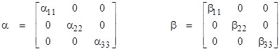
There is, however, a special circumstance in which the bra-ket operation does possess the multiplicative property, namely, in the case when both α and β are diagonal and A is an eigenvector of both of them. To see this, consider the two diagonal matrices

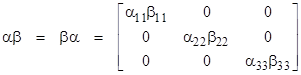
The product of these two observables is

Note also that in this special case the multiplication of operators is commutative. Now, taking the state vector to be the normalized eigenvector [0  1  0] for example, we get

Therefore, following Dirac’s reasoning, we are justified in treating the number <A|α|A> as the unique result of measuring the observable α for a system in state A provided that A is an eigenvector of α, in which case the result of the measurement is the corresponding eigenvalue of α.

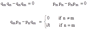
From this it follows that quantum mechanics would entail no fundamental indeterminacy if it were possible to simultaneously diagonalize all the observables. In that case, all observables would commute, and there would be no “Heisenberg uncertainty”. However, we find that it is not possible to simultaneously diagonalize the operators corresponding to every pair of observables. Specifically, if we characterize a physical system in Hamiltonian terms by defining a set of configuration coordinates q₁, q₂, … and the corresponding momenta p₁, p₂, …, then we find the following commutation relations

These expressions represent the commutators of the indicated variables, which are closely analogous to the Poisson brackets of the canonical variables in classical physics. These commutators signify that each configuration coordinate q_j is incompatible with the corresponding momentum p_j. It follows that we can transform the system so as to diagonalize one or the other, but not both.

Shortly after Heisenberg created matrix mechanics, Schrödinger arrived at his theory of wave mechanics, which he soon showed was mathematically equivalent to matrix mechanics, despite their superficially very different appearances. One reason that the two formulations appear so different is that the equations of motion are expressed in two completely different ways. In Heisenberg’s approach, the “state” vector of the system is fixed, and the operators representing the dynamical variables evolve over time. Thus the equations of motion are expressed in terms of the linear operators representing the observables. In contrast, Schrödinger represented the observables as fixed operators, and the state vector as varying over time. Thus his equations of motion are expressed in terms of the state variable (or equivalently the wave function). This dichotomy doesn’t arise in classical physics, because there the dynamic variables define the state of the system. In quantum mechanics, these two things (observables and states) are two distinct things, and the outcome of an interaction depends only on the relationship between the two. Hence we can hold either one constant and allow the other to vary in such a way as to give the necessary relationship between them.

This is somewhat reminiscent of the situation in pre-relativistic electrodynamics, when the interaction between a magnet and a conductor in relative motion was given two formally very different accounts, depending on which component was assumed to be moving. In the case of electrodynamics a great simplification was achieved by adopting a new formalism (special relativity) in which the empirically meaningless distinction between absolute motion and absolute rest was eliminated, and everything was expressed purely in terms of relative motion. The explicit motivation for this was the desire to eliminate all asymmetries from the formalism that were not inherent in the phenomena. In the case of quantum mechanics, we have asymmetric accounts (namely the views of Heisenberg and Schrödinger) of the very same phenomena, so it seems natural to suspect that there may be a single more symmetrical formulation underlying these two accounts.

The asymmetry in the existing formalisms seems to run deeper than simply the choice of whether to take the states or the observables as the dynamic element subject to the laws of motion. This fundamentally entails an asymmetry between the observer and the observed, whereas from a purely physical standpoint there is no objective way of identifying one or the other of two interacting systems as the observer or the observed. A more suitable formalism would treat the state of the system being “observed” on an equal footing with the state of the system doing the “observing”. Thus, rather than having a matrix representing the observable and a vector representing the state of the system being observed, we might imagine a formalism in which two systems are each represented by a matrix, and the interaction of the two systems results in reciprocal changes in those matrices. The change in each matrix would represent the absorption of some information about the (prior) state of the other system. This would correspond, on the one hand, to the reception of an eigenvalue by the observing system, and on the other hand, to the “jump” of the observed system to the corresponding eigenvector. But both of these effects would apply in both directions, since the situation is physically symmetrical.

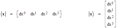
In addition to it’s central role in quantum mechanics, the bra-ket operation also plays an important role in the other great theory of 20th century physics, namely, general relativity. Suppose with each incremental extent of space-time we associate a “state vector” x whose components (for any given coordinate basis) are the differentials of the time and space coordinates, denoted by super-scripts with x⁰ representing time. The bra and ket representatives of this state vector are

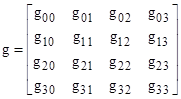
Now we define an “observable” g corresponding to the metric tensor

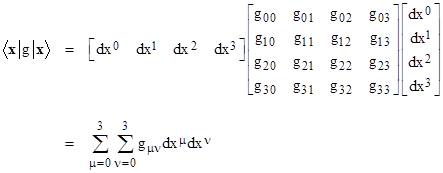
According to the formalism of quantum mechanics, a measurement of the “observable” g of this “state” would yield, on average, the value

This is just the invariant line element, which is customarily written (using Einstein’s summation convention) as

However, unlike the case of quantum mechanics, the elements of the vector x and operator g are purely real (at least in the usual treatment of general relativity), so complex conjugation is simply the identity operation. Also, based on the usual interpretation of quantum mechanics, we would expect a measurement of g to always yield one of the eigenvalues of g, leaving the state x in the corresponding eigenstate. Applying this literally to the diagonal Minkowski metric of flat spacetime (in geometric units so that c = 1), we would expect a measurement of g on x to yield +1, -1, -1, or -1, with probabilities proportional to (dx⁰)², (dx¹)², (dx²)², (dx³)² respectively. It isn’t obvious how to interpret this in the context of spacetime in general relativity, although the fact that the average of many such measurements must yield the familiar squared spacetime interval (ds)² suggests that the individual “measurements” are some kind of quantized effects that collectively combine to produce what we perceive as spacetime intervals.

Return to MathPages Main Menu