On de Bruijn Grids and Tilings

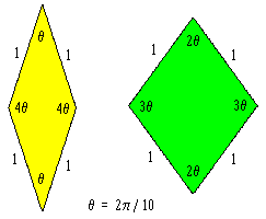
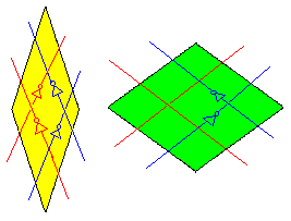
In a note on aperiodic tilings we discussed how the inflation and substitution method can be used to generate arbitrarily large Penrose tilings. A different – and very striking – approach was devised by the Dutch mathematician N. G. de Bruijn in 1981. It is most easily described in terms of the “rhombus” form of Penrose tiles, i.e., the two proto-tiles are both four-sided parallelograms with unit edge lengths and interior angles in the proportions 1:4 and 2:3 as shown below.

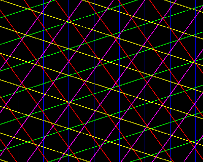
Since all the edges have the same length, the edge lengths impose no restriction on how we may adjoin tiles. At this stage, the only requirement is that the vertex angles meeting at any point must sum to 2π = 10θ. In other words, only the angles of intersection are important, not the metrical distances, so any conformal mapping of the edges would be acceptable. This beautiful insight enables us to determine a complete aperiodic tiling of the plane simply by mapping from the intersections of five sets of parallel grid lines, at unit intervals, directed at angles of 2π/5, as illustrated below.

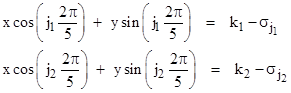
The equation of the kth grid line in the jth set is

where σ_j is an offset of the jth set of lines in the direction normal to the lines. In order to map the intersections of these lines to the joined edges of a tiling, we need to ensure that no more than two lines meet at any given point. This can be achieved by suitable choice of the offsets. To show this, we first note that every pair of lines (from two different sets) intersects at exactly one point, which can be found by simultaneously solving the equations

Solving each of these for the x coordinate of the intersection point and setting the those values equal to each other, we get the following equation for the y coordinate of the intersection point

where, for brevity, we have defined the symbols

Now, if a third line (not parallel to either of the first two), characterized by k₃ and σ₃,  intersects with these two lines at this same point, we would necessarily have

It follows that μ₁, μ₂, μ₃ are proportional to c₁, c₂, c₃. The values of cos(2πj/5) for j = 0 to 4 are

respectively, so each ratios of μ values must equal a ratio of two of these cosine values. The ratio of any two of these cosines is either irrational or unity. We can exclude the possibility of a unit ratio by simply making the σ values distinct and non-complementary, so that the μ values are all distinct. We can also exclude the possibility of an irrational ratio by choosing rational values of σ (and hence of μ). Therefore, if the values of σ_j are all rational and distinct, and no two of them sum to an integer, it is impossible for three of the grid lines to intersect at any point.

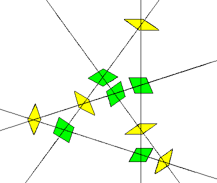
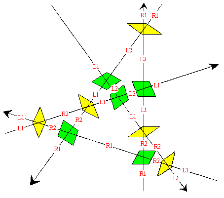
At each intersection between two grid lines we can construct a rhombus with faces normal to those grid lines. This is illustrated in the figure below for a typical region of the grid.

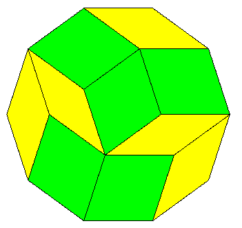
Notice that there are just two kinds of intersections, corresponding to the wide rhombus and the thin rhombus discussed previously. The grid lines provide a complete mapping for a tiling of the plane, and we can now assemble the tiles in the indicated pattern to give the coherent cluster shown below.

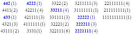
The entire tiling is non-periodic, but of course we can also tile the plane periodically with one or both of the rhombi. To make these proto-tiles into an aperiodic set (i.e., a set that tiles only non-periodically) we need to impose some local restrictions on how the tiles may be adjoined to each other. With no such restrictions, the number of distinct vertices (up to rotation) equals the number of partitions of 10 into the numbers 1, 2, 3, 4. The 23 such partitions are listed below, along with, in parentheses, the number of distinct (up to rotation and reflection) orderings of each partition.

Thus there are 54 distinct possible vertices if we place no other restrictions on them. For example, the partition “1111111111” represents ten of the thin rhombi meeting at a single vertex. In the context of a de Bruijn grid this vertex would correspond to a face with ten sides, each intersection being of two lines whose angles differ by just π/5. Such a face is clearly possible in a grid if we are free to choose the offsets σ_j arbitrarily. However, if we remove one degree of freedom by requiring that

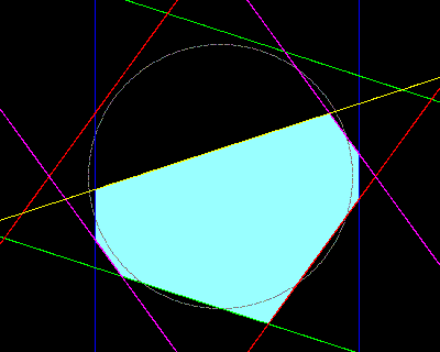
then it’s not too difficult to show that the grid cannot contain any faces of the form “1111111111”. The closest we can get is to select a single point (say, the origin), and position the sets of grid lines so that the point is mid-way between two consecutive lines in each set. But this requires offsetting each set by ±1/2, so the offsets do not sum to zero. If we offset just four of the sets by ±1/2, the fifth set must be offset by 0 (modulo 1), so it bisects the face formed by the other sets. We can slightly shift the first four offsets so that the fifth is non-zero, but it’s not hard to see that the maximum number of sides of a face in the grid with the above summation condition on the offsets is seven, as shown by the highlighted region in the figure below.

The angles of the tiles meeting at the vertex corresponding to this grid face are 2211211, which is one of the four “2221111” partitions highlighted in blue in the preceding list. By shifting the line sets, always ensuring that the offsets sum to zero, we can show that the only possible faces that can appear in such a grid corresponds to the following seven cycles of vertex angles meeting at a given point of the tiling:

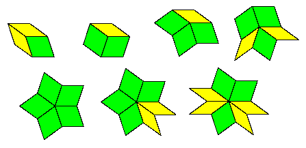
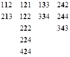
The seven corresponding partitions of ten are highlighted in blue in the previous list. This shows that the only vertices in a tiling produced in this way are (up to rotations) of the seven forms shown below.

Notice that each “1” appears in the middle of either the sequence 112 or 213 (or the reversals). Likewise we can list the possible neighborhoods of each angle as shown below.

Thus a “1” angle cannot be adjacent to a “4” angle in the cycle of angles at any vertex, and a “3” cannot be adjacent to a “2”. Also, each “3” must be adjacent to another “3”, and so on. Also, since five green tiles can all fit together at a vertex (22222), the edges of the green rhombus forming a given “2” vertex must all be compatible (noting that five is odd, so the edge types can’t alternate). Furthermore, since the yellow tile can mate with those green edges, the edges of a yellow rhombus forming a given “4” vertex must be of this same type, and the other two edges must mate with the opposite edges of the green rhombus.

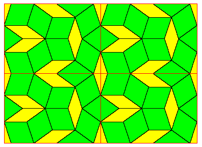
By imposing these local joining requirements on the tiles we do not affect the ability to form non-periodic tilings by means of de Bruijn grids, but we do interfere with the ability to form periodic tilings. It should be noted, however, that restricting ourselves to just the above vertex types we do not preclude a periodic tiling. This is shown by the arrangement below.

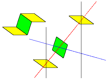
So, in order to preclude any periodic tiling, we need some stronger restrictions. Notice that the above periodic pattern could never arise from a de Bruijn grid, because it contains occurrences of two yellows adjoined to a green in the way shown in the left side of the figure below.

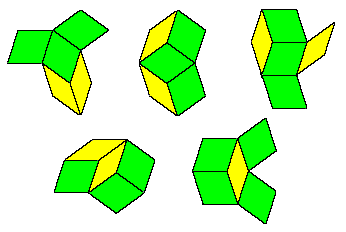
The right side of this figure shows the arrangement of grid lines that would be required to give this cluster of tiles, but this arrangement cannot occur in a de Bruijn grid because the red line passing between two black lines intersects only one other line, namely the blue line. Since a de Bruijn pentagrid has equally-spaced lines in all five directions, the red line must intersect with each of the other colored lines at least once between every consecutive pair of black lines (because the red and black lines are angularly adjacent). Therefore, the above cluster of two yellows and a green tile cannot occur. In fact, if we define the word “neighborhood” to signify a tile together with its four adjacent tiles, then by similar reasoning we can show that a de Bruijn grid permits only the five neighborhoods (up to rotations and reflections) shown below.

Every other neighborhood is precluded by the conditions satisfied by the grid lines. Thus, up to rotation and reflection, each thick tile can have one of only three neighborhoods, and each thin tile can have one of only two neighborhoods. These facts provides a strong technique for extending the tilings, consistent (at least locally) with the limitations imposed by the de Bruijn grid. For example, by considering the possible neighborhoods of the non-central thin tile in the lower left hand cluster above, it’s clear that it can only be a reflection of the neighborhood of the central tile, because this is the only neighborhood for a thin tile such that one of the neighbors is also a thin tile.

To more conveniently encode the neighborhood restrictions, suppose we regard each tile as a logical operator that relates a set of binary inputs on one edge to a set of binary inputs on the opposite edge. In particular, suppose we define the tile operators as shown below.

For convenience, we will let L, R denote the “red” binary values, and 0, 1 denote the “blue” values. We can then assign values to some location on each grid line, and the values at every other point on that line are determined by the operators (nothing that these are reversible functions). For example, we get the following network of values for the “exploded” tiling discussed previously.

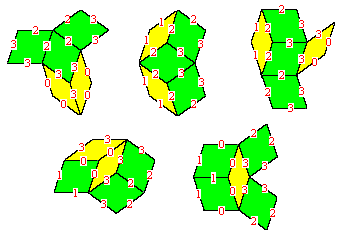
As we proceed along each line (in either direction), both the letter and the numeral are toggled by each yellow tile, whereas only the numeral is toggled by each green tile. Notice the four edges of any given green tile all have the same letter, and the numerals are the same for each pair of edges meeting at the narrow vertex, and toggled for each pair of edges meeting at the wide vertex. On the other hand, for any given yellow tile, the two edges meeting at a wide vertex have identical letters and numerals, toggled on the opposite two edges. We can show that these attributes persist throughout the entire tiling, by simply considering each of the five possible neighborhoods, as shown below, with the encoding 0 = L1, 1 = L2, 2 = R1, and 3 = R2.

In this figure we have arbitrarily chosen attributes for the edges of the central tile, consistent with the stated conditions, and then chosen the surrounding tiles so that the conditions are also satisfied for those tiles, while obeying the logical operations of each tile. We can likewise show that all seven of the possible vertex arrangements are consistent with this conditions. (One of the seven is consistent in two distinct ways, as discussed below.)

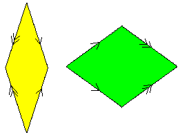
It’s also worth noting that, in the grid layout, the positive senses of the two grid lines intersecting in a green tile are such that the minor angle always encloses a 3θ vertex, whereas the minor angle between the positive grid lines intersecting in a yellow tile always encloses a 1θ vertex. As a consequence, we can associate the “blue” logical variable with a direction along an edge relative to the positive sense of the perpendicular grid line, and this will make all the tiles (of a given type, i.e., green or yellow) identical up to rotation and reflection. The “red” logical variable can be regarded as signifying one of two types of directed edges. This gives the well-known matching rules for Penrose rhombus tiles:

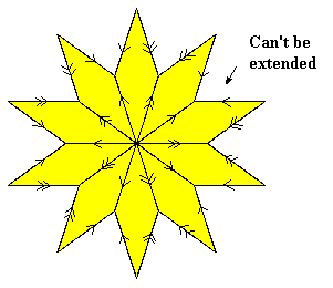
It’s easy to see that these arrows encode the same restrictions as the logical operators. For example, passing from one edge to the opposite edge of a yellow tile toggles both the direction and the type of the arrow, whereas passing from one edge to the opposite edge of a green tile toggles just the type of the arrow. Hence any tiling that can arise from a de Bruijn grid can be implemented using tiles of this type. Conversely, it can be shown that any complete tiling that can be produced from tiles with these matching conditions corresponds to a tiling that arises from a de Bruijn grid. The qualifier “complete” is important, because we can clearly construct finite clusters of tiles of this type that cannot occur in a de Bruijn grid.  For example, a star consisting of ten yellow tiles satisfies the immediate matching rules, as shown below.

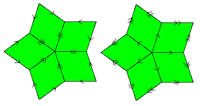
However, this cluster cannot appear in a complete tiling of the plane – nor in a de Bruijn grid – because it has edges that cannot be extended, such as the one indicated. No matching tile can fit into that region, so this is not one of the allowed vertices in a complete tiling. Of the seven vertex types that actually do occur in a complete tiling, six of them have unique arrow arrangements. The exception is the five-point star consisting of five green tiles, which can occur with either of the two distinct arrow arrangements shown below.

There’s an interesting analogy between the tile “operator variables” discussed above and potential fields in physics. For each tile we defined a reversible two-bit operator for each pair of opposing edges. These two operators were independent, and nothing prevents stringing together any number of such operators in sequence, so we have five independent sequences of operators, criss-crossing each other in the five directions, but not interacting with each other. However, we found that, with a certain assignment of variables in each of those five directions, the operators of each tile were effectively synchronized, such that given the value of the (two-bit) logical variable on any edge, the values on the other three edges (not just the opposite edge) are fully determined. Now we can proceed in any direction through a tile, so we have a logically unified two-dimensional space, and consistency requires that the composition of operators along each possible path between two given edges must yield the same overall operation. The values of the variable at each edge are arbitrary, since only the change of the variable from one edge to another has significance. This is quite analogous to potential fields in physics, for which the absolute value of the potential is unimportant, but it is required that the change in potential when proceeding from one given point to another is well-defined, independent of the path that is followed.

Since the logical operations we used are restricted to negation, which is reversible, we effectively require “even parity” over any closed loop in the tiling. There are six ways of traversing a tile, since we can go from any one of the four edges to any of the others. Letting the edges of a given tile be denoted by a,b,c,d, we can characterize the operation of each tile on each bit of the field variable by three bits of information, such as by assigning either +1 or -1 to each of the pairs ab, ac, ad. This is sufficient to determine the signs of the other three traversals, since we have (ab)(ac) = a²bc = bc, and so on.

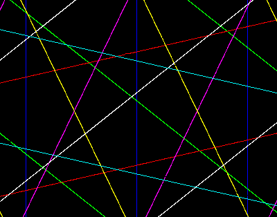
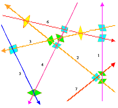
The above discussion focused on grids and tilings based on the pentagonal angle π/5, but much of it can be generalized to quasi-periodic tilings based on other polygonal angles. For example, using the septagonal angle π/7 we can construct a de Bruijn grid just as before, except now there are seven (instead of five) families of parallel grid lines, as shown below.

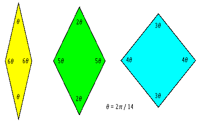
As before, we chose offsets so that no more than two lines intersect at any given point. In this case there are three different kinds of intersections (up to rotations and reflections), so the rhombic proto-tiles with edges perpendicular to the intersecting lines must have the following three shapes.

To construct a tiling we assign a suitable one of these prototypes to each intersection in the grid. The figure below shows the assignments for a small section of the grid.

Bringing these thirteen tiles together in the indicated way, we get the following arrangement:

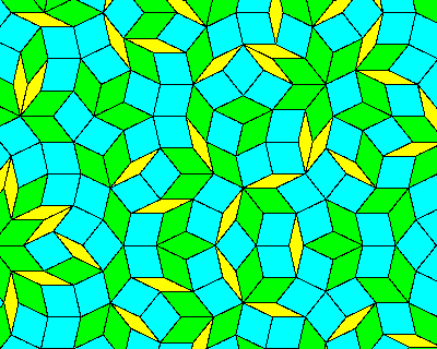
The septagrid encodes instructions for tiling the complete plane with quasi-septagonal symmetry using the three rhombic proto-tiles. Adding more of the tiles from the same grid construction, we get a tiling exemplified by the region shown below.

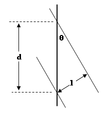
Notice that in the region of 205 tiles shown above we can see (at least a portion of) 40 yellow tiles, 73 green tiles, and 92 blue tiles. Just as the asymptotic ratio of the number of thick and thin rhombs in Penrose tilings is the golden proportion 1.618…, we can easily determine the proportions of the three different rhombs in this septile pattern by considering the frequency with which any given grid line is intersected by uniformly spaced lines at angles of π/7, 2π/7, and 3π/7, as indicated below.

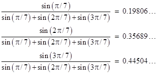
The asymptotic frequency of intersections is inversely proportional to the distance between the intersections, so it is proportional to 1/d = sin(θ). Consequently the numbers of yellow, green, and blue tiles in a septiling are asymptotically proportional to

This already agrees quite well with the numbers of tiles visible in the above image, where we counted

A nice interpretation of the grid procedure for determining quasi-periodic tilings is to notice that we can assign to each point of the plane seven coordinates, measured along the seven principle normal directions of the grid lines. Of course, there are really only two degrees of freedom, but we can still conceive of this two-dimensional plane embedded in a seven-dimensional space. Furthermore, each “face” of the septagrid can be associated with a lattice point (i.e., a point with integer coordinates) in the seven-dimensional space, because each face exists between two discrete lines in each of the seven families of grid lines. Moreover, as we move from one face of the grid to a neighboring face, we cross over one grid line, and in doing so we move one unit in the corresponding principle direction to get to the next vertex of the tiling. Thus the vertices of the tiling are really just projections of the “nearest” lattice points in seven-dimensional space onto a two-dimensional slice through that space.

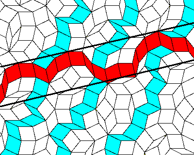
With this in mind, we can see one fairly simple way of drawing the tiling corresponding to any given septagrid (i.e., to any given offset vector γ_i with i = 0,1,..,6). For any desired region of the plane we can scan each point with polar coordinates r,θ, and compute the coordinates for the lattice point corresponding to that face in which that point resides as follows

where the brackets signify the largest integer less than the enclosed quantity. Of course, if we scan the region uniformly, we will find many points in the same face, so we need save only one occurance of each distinct lattice point. These are the lattice points that neighbor our plane. Once we have found all the distinct nearby lattice points in this way, the plane coordinates of the tiling vertex corresponding to each of those lattice points are given by

Given the list of vertices, we can then draw a line from each vertex to every other vertex that is a distance of 1 unit away, thereby giving a complete picture of the tiling in the subject region.

This kind of tiling, and the corresponding tilings with quasi-N-fold symmetry for N = 9, 11, 13, etc., seem to be rarely mentioned in popular discussions of tilings. It would be interesting to see if any simple “local” matching rules exist which would preclude any periodic tiling. We might begin by enumerating all possible vertices and all possible neighborhoods. We could also compute all the possible invertible logic operations that yield even parity around every loop in the tiling. Regardless of whether there exist simple local matching rules to preclude periodic tiling of these proto-tiles, it seems that nothing would prevent crystal formation with this quasi-septagonal symmetry.

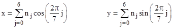
It’s worth emphasizing that, even the usual matching rules for Penrose rhombs could be considered “non-local” in the sense that they allow tiles to be adjoined in ways that lead to interferences only at some later stage and distant location. The simplest example of this is the fact that the matching rules allow ten of the thin rhombs to be adjoined at a common vertex, even though it isn’t possible to extend this combination of tiles without violating the matching rules (as described previously). In general it seems that “matching rules” could be expressed in many different forms, with the only requirement being that we must ensure that each of the principle directions is introduced. For example, we could impose the requirement that every “ribbon” stays within a certain distance of its axis, i.e., the mean line perpendicular to each pair of opposite edges, as indicated in the figure below.

A ribbon in each of the principle directions must occur at uniformly spaced intervals. Since there are no perfectly periodic patterns with n-fold rotational symmetry for n = 7, 9, 11, etc., the requirement that each of the ribbons stays close to its axis is sufficient to ensure non-periodicity.

Return to MathPages Main Menu