The Ergodic Hypothesis and Equipartition of Energy

One of the most important principles of physics is the principle of the equipartition of energy, according to which the energy of a system will tend to distribute itself equally over all the degrees of freedom of the system. However, the equipartition of energy can only be asserted with several qualifiers and provisos – even classically. The equipartition principle relies on the ergodic hypothesis, which basically asserts that a system’s path in phase space on a surface of constant energy will, in the long run, visit each region of that surface equally often. To express this more precisely, recall that the dynamical state of a system with n degrees of freedom can be represented by a point in the 2n-dimensional phase space whose axes are the n generalized coordinates q_i and the n generalized momenta p_i of the system. The total energy (kinetic plus potential) of the system can be expressed as a function (called the Hamiltonian) of the generalized coordinates and momenta. An isolated system with a given amount of energy is confined to that energy surface in phase space. To each small region on that surface we can assign a weight factor proportional to the volume (of phase space) swept out by that region for an incremental change in energy. Using this weight factor we can then evaluate the mean values of any variable X(q,p) on the surface. This is called the phase average of X, denoted by <X>. In addition, we can consider the path of an actual system through phase space as a function of time, and assuming the time-average of X converges on a single value, we can denote this value as . The ergodic hypothesis is that

Of course, it’s easy to conceive of circumstances in which this hypothesis doesn’t hold. For example, the energy surface in phase space may consist of multiple separate surfaces, making it impossible (classically) for a system to jump from one to the other. For another example, the path of the system may be periodic, visiting only points along some finite loop. More subtly, a system may evolve in an orbit that never precisely repeats, but it may nevertheless be confined to an “attracting orbit” within a sub-region of the surface. The ergodic hypothesis also requires that all the degrees of freedom be dynamically coupled, and that we exclude “special” initial conditions that lead to restricted orbits. Even for circumstances in which the ergodic hypothesis applies, the time scale over which the system can be expected to visit all regions may be so enormous that, for practical purposes, the ergodic hypothesis is not very relevant. (In view of all these exceptions, we might summarize by saying that the ergodic hypothesis is always valid, except when it isn’t.)

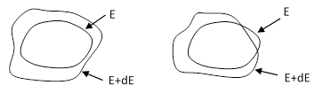
Another consideration regarding the ergodic hypothesis is the different ways in which a surface of constant energy may change as a function of the energy. Two possible cases are depicted below.

The weight factor assigned to each region on the surface E is proportional to the “thickness” between E and E+dE in that region, and in the left-hand figure this thickness is always non-zero and has the same sign, so it provides a well-defined density distribution. However, in the right-hand figure the two surfaces intersect, so that the “volume” between them has two different signs, and at the points of intersection the swept volumes for the regions around those points go to zero. Is it possible for surfaces of constant energy to exhibit this kind of behavior in phase space? If it is, then it’s not clear how the weight distribution could be normalized. Also, the locus of points with zero weight might be barriers, undermining the premises of the ergodic hypothesis.

All the same qualifiers on the applicability of the ergodic hypothesis apply to the principle of the equipartition of energy as well. In addition, from a physical standpoint, the “degrees of freedom” of any physical system are somewhat ambiguous and context-dependent, nut just because of non-linear modes, but also because there are no fully isolated systems. It has been noted by others that every atom is dynamically coupled with every other atom in the universe, at least by means of electromagnetic and gravitational fields. (which have infinite range). Gravitation, in particular, cannot be shielded, and couples to all forms of mass-energy. Nevertheless, equipartition of energy is one of the most important principles in both classical and quantum mechanics.

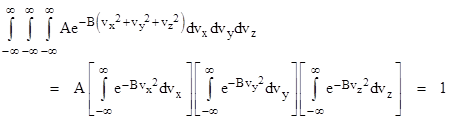
Usually we neglect the long-range interactions and focus on just the local energy modes that are quadratic in the associated coordinate or momentum. The usual generic “proof” of the equipartition of energy in this context is based on the premise that each of the generalized coordinates and momenta are distributed according to a Maxwell-Boltzmann distribution. The actual justification for this premise in each case is rarely given. Instead, expositions often avail themselves of a clever argument given by Maxwell for the distribution of the speeds of molecules in a gas. He sought a distribution density function ϕ(v_x,v_y,v_z) that would represent the fraction of molecules with speeds in the incremental window v_x to v_x + dv_x, v_y to v_y + dv_y, and v_z to v_z + dv_z.  Hence the triple integral of ϕ over all possible speeds must equal 1, i.e.,

At this point Maxwell referred to an analysis he had performed on the scattering angles of colliding spheres, which had led him to conclude that all directions of recoil are equally probable (in a gas of randomly moving particles). From this he argued that all directions of motion are equally probable, and therefore the density must depend only on the magnitude of the speed, not on its individual components. For example, the density ϕ(1,0,0) must be the same as the density ϕ(0,1,0), because there is no inherent difference between the x and y directions. Hence there is a uni-variate function f such that

Furthermore, since the distributions in the x, y, and z directions are statistically independent, Maxwell asserted that the density for any given speed must be proportional to the product of the densities of its components, i.e.,

for some constant κ. The only continuous real-valued function such that f(a+b) = f(a)f(b) is the exponential function, so Maxwell concluded that the distribution of speeds must be of the form

where α and β are constants. The minus sign in the exponent is chosen because a positive exponent would not give a convergent integral. The value of α can be inferred from the requirement for equation (1) to be satisfied. Substituting from (2) into (1) gives

Each of the integrals is equal to (π/β)^1/2, so we have

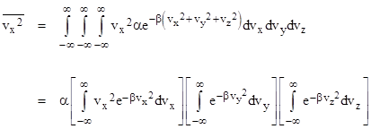
Furthermore, given the density distribution (2) of velocities, we can compute the mean values of any variables that depend only on the velocity. For example, the mean value of v_x² is given by

Again the second two integrals each equal (π/β)^1/2, and in addition the first integral evaluates to (π/β)^1/2/(2β), so we have

By symmetry we get exactly the same mean values of v_y² and v_z², and we know the mean value of |v|² is simply the sum of the mean values of the squared components, so we have

To relate the constant β to other thermodynamic variables, consider a single perfectly elastic monatomic particle of mass m confined in a cubical box of size L x L x L with perfectly elastic walls, and suppose the components of the particle’s velocity at a particular instant are v_x, v_y, v_z. Note that collisions with the walls in the y and z directions have no effect on the x component of the particle’s motion, so the particle will strike each of the walls normal to the x axis once every 2L/vx seconds, imparting a momentum of 2mv_x on each of these collisions (because the particle impacts the wall at speed v_x and departs at speed –v_x).  Hence the average force (momentum per time) imparted to each of these walls is mv_x²/L. By the same reasoning, the mean force applied to each of the walls normal to the y axis is mv_y²/L, and to each of the walls normal to the z axis is mv_z²/L.

Now, if we have N such particles in the box, and we note that the pressure on each wall is the total force divided by L², we see that the pressure on the walls will be

where the over-bar denotes the average. Since Nm/L³ is the density, ρ, these expressions can be written as

Arguing that there is no preferential direction, the average velocity components in the three directions are equal (which implies that the average kinetic energies of a molecule in each of the three directions are equal), so the pressures on the walls are equal, and we have

(It’s debatable whether the particle velocities really are perfectly isotropic when enclosed in a cubical container, but in practice this turns out to be a fair assumption for most purposes.) Recall that p = ρRT = ρ(k/m)T for an ideal gas, where ρ is the density, R is the gas constant, T is the temperature, m is the mass of a single molecule, and k is Boltzmann’s constant. Hence we have

Combining this with equation (3) and solving for the constant β gives the result

Inserting the values of a and b into equation (2), we arrive at the Maxwell-Boltzmann distribution

Since R = k/m, this can be written in the form

Thus the numerator of the exponent is just the sum of the translational kinetic energies in the three directions. We already know, from the previous equations, that the mean kinetic energy in each of the three directions is kT/2 (although it’s arguable that this was more or less an assumption), and this can easily be verified by integrating with the density function.

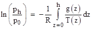
Moreover, it is argued that every energy mode has a distribution density function of the same form as (4), from which it follows that if the energy is a quadratic function of either the generalized coordinates or the generalized momenta, then the mean value of that energy mode (in equilibrium) is kT/2. This is the principle of equipartition of energy. It may be somewhat surprising at first that all the different species of energy modes, potential as well as kinetic, all exhibit a Boltzmann distribution. For the case of gravitational potential energy in an ideal gas this can be established by a simple argument. As discussed in Geophysical Altitudes the pressure in a column of gas at the height z = h compared to the pressure at z = 0 is given by

where g(z) and T(z) are the gravitational acceleration and temperature (respectively) at the height z. If we assume the temperature and the acceleration of gravity are constant over the range of interest, then the integral is just gh/T and we have

Since p = ρRT, and since mgh is the difference in potential energy Δε between molecules at the heights z = 0 and z = h, this relation can be written as

Thus the density of molecules has a Boltzmann distribution over the range of potential energies, just as they do over the range of translational kinetic energies. For the case of potential energy we see that the distribution arises due to the simple fact that the molecules need to be more densely populated at the lower energy regions in order to produce the pressure to support the higher energy regions.

This makes it at least plausible that all the energy modes have a Boltzmann distribution, and therefore the mean value of the energy of each mode is kT/2. To show that this is mathematically consistent, let’s consider a more general class of energy modes, each of the form aq² or bp² where “a” and “b” are constants, q is a generalized coordinate, and p is a generalized momentum (not to be confused with pressure). For example, the translational kinetic energy of a particle of mass m is ε_T = p²/(2m), and the potential energy stored in a spring is ε_S = Cq²/2 where C is the spring constant. The Hamiltonian of the system is the total energy as a function of the generalized coordinates and momenta, so for a mass-spring system we have

The distribution is assumed to be of the Boltzmann form, so we have

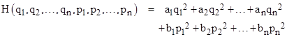
More generally, consider the Hamiltonian

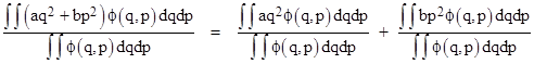
The mean value of any of the energy terms is found by an expression of the form

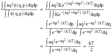
where the integrals are evaluated from negative to positive infinity. The first term on the right side is

Since this result doesn’t depend on the value of the coefficient “a”, it clearly applies to every quadratic energy term in the Hamiltonian, consistent with the claim that each degrees of freedom has the same average energy.

Of course, this result actually follows immediately from the premise that every energy mode has a Boltzmann distribution with parameter kT. In addition, we tacitly invoked the ergodic hypothesis by arguing that the system’s path on the energy-surface within phase space will, in the long run, visit each accessible region with a frequency proportional to the volume of the region. Naturally if the system’s path is periodic or bounded within a restricted orbit, or if the energy modes are not dynamically coupled, the ergodic hypothesis doesn’t apply. Furthermore, the actual energy modes of real physical systems are generally not simply quadratic. In addition, as alluded to previously, the tacit assumption that energy can take on any real value turns out to be false, due to quantum effects. For all these reasons, the specific heats of substances with complicated energy modes do not generally agree with the simplistic classical prediction. (They generally vary with temperature, and approach the classical prediction only at very high temperatures.)

It’s interesting that Maxwell’s deduction of the velocity distribution function works in three or two dimensions, but not in one dimension. Sure enough, it can be shown that the velocity distribution in one dimension does not approach the Maxwell distribution. This shows that the directional scattering which occurs in two or more dimensions is crucial. Regarding this distribution, Maxwell commented

It appears from this proposition that the velocities are distributed among the particles according to the same law as the errors are distributed among the observations in the theory of the “method of least squares”. The velocities range from 0 to ∞, but the number of those having great velocities is comparatively small.

Maxwell went on to show that, if two populations of particles (with different masses) are mixed, they will approach an equilibrium condition in which the average kinetic energy of each species of particle is the same. He might have made use of the mean-value integration presented above for the combined Hamiltonian, but instead he presented a pictorial and algebraic proof, which not only showed the equilibrium configuration but also gave a quantitative indication of how rapidly a system of particles would approach equilibrium.

Let M and m be the masses of the particles in the two populations, and let v₀ and u₀ be, respectively, the mean speeds of these two populations of particles prior to any collisions between the two populations. After one of the particles from the first population has collided with one of the particles from the second population, let v₁ and u₁ denote the new average speeds of the particles. He had shown previously that if v₀ and u₀ are the mean absolute speeds, then the mean relative speed between the two sets of particles is given by

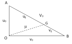
This can be represented pictorially as the lengths of the edges of a right triangle as shown below. (Note that this is not a space vector diagram; the directions of the segments do not signify directions in space, but rather degrees of correlation.)

The mean speed of the center of gravity of two particles, one from each population, corresponds to the length of the interval from O to G, where the point G is chosen with the appropriate weighting, i.e., such that the ratio of the segments GA and GB is inversely proportional to the masses. Combining the requirements u_g/v_g = M/m and u_g + v_g = V₀, we get

We can now solve for the length m of the segment OG, noting that this segment has orthogonal components u_gv₀/V₀ and v_gu₀/V₀ (by similar triangles) to give

After these two particles collide, their speeds relative to their center of gravity will be unchanged in magnitude, but the axis of their mutual recoil will be from a uniform distribution relative to the direction of their center of gravity (as Maxwell had shown previously). Therefore, the mean result is represented by placing the recoil speeds perpendicular to the segment representing the center of gravity, as shown in the figure below.

Consequently, the mean speeds of the two particles following the collision are equal to the lengths of the segments Oa and Ob, which are denoted by u₁ and v₁ in the figure. Since OGa and OGb are right triangles, we know that

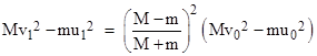
and therefore we have

This shows that the difference between the kinetic energies of the two particles is less following the collision than it was prior to the collision. The same argument applies to every collision, so the difference drops exponentially to zero. From this Maxwell concludes that the mean translational kinetic energies of any number of monatomic particles of any masses approach equality at equilibrium. Naturally this is consistent with the previous demonstration.

Return to MathPages Main Menu