Geophysical Altitudes

Four distinct kinds of "altitude" are commonly used when discussing the vertical heights of objects in the atmosphere above the Earth's surface. The first is simple geometric altitude, which is what would be measured by an ordinary tape measure. However, for many purposes we are more interested in the pressure altitude, which is actually an indication of the ambient pressure, expressed in terms of the altitude at which that pressure would exist on a "standard day". Similarly, the density altitude is an indication of the ambient air density, expressed in terms of the altitude at which that density would exist on a "standard day". Finally, there is the so-called geopotential altitude, which is really a measure of the specific potential energy at the given height (relative to the Earth's surface), converted into a distance using the somewhat peculiar assumption that the acceleration of gravity is constant, equal to the value it has at the Earth's surface.

The geometric altitude is fairly self-explanatory, but is often difficult to measure accurately in real situations (such as from an airplane), because of irregularities in the terrain. Moreover, for the purposes of operating air-breathing equipment (such as human lungs or jet engines), what really matters is ambient pressure, which of course corresponds to the density of the ambient air. If we let z denote the geometric altitude above sea level, and if we let p(z), r(z), and g(z) denote the atmospheric pressure and density and the acceleration of gravity at the height z, then the rate of change of pressure with respect to geometric altitude is given by the "hydrostatic equation"

Also, treating air as an ideal gas, we have

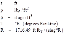
where T(z) is the temperature and R is gas constant for air. One possible set of units for these quantities is

Combining equations (1) and (2) gives

Integrating from z = 0 (sea level, where the pressure is p₀) to z = h (where the pressure is p), we have

Now, for aviation purposes we are typically confined to the region below about 45000 ft geometric altitude, and the acceleration of gravity at that height is not very different than at sea level, so to a good approximation we can treat g(z) as a constant. Because of the oblateness of the earth, this varies appreciably at different latitudes, from about 32.02 to 32.26 ft/sec², but for our purposes, we can use a value of g = 32.17277 ft/sec².  (We will explain below the reason for selecting this precise value.)

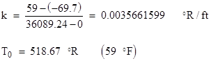
Also, the "standard day" temperature profile is defined to be 59 F at sea level, and dropping linearly to −69.7 F at the tropopause, which is at 36089.24 feet (11000 meters) above sea level. Above this altitude the standard day temperature is constant, up to well past 50000 ft. Therefore, over the range from sea level to the tropopause we can write equation (4) as

where

Evaluating the integral in (5) and solving the resulting expression for h gives

With p₀ = 14.696, this expression for h is defined as the pressure altitude corresponding to the ambient pressure p, for all values of p greater than or equal to 3.2825, which represents the standard tropopause. Inserting the values of the constants, this gives the formula for pressure altitude as a function of ambient pressure

For pressures less than 3.2825, equation (5) gives

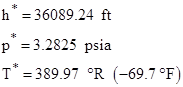
where asterisks indicate conditions at the tropopause (on a standard day)

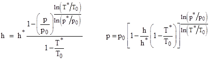
Solving (8) for h gives the formula for pressure altitude as a function of ambient pressure for conditions above the tropopause

Inserting the values of the constants gives

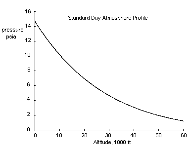
A plot of ambient pressure versus pressure altitude is shown below.

Needless to say, this derivations depends on the particular temperature profile that we have assumed. We used the "standard day" profile based on the 1962 Geophysical Survey. There are also conventional definitions of "Hot Day" and "Cold Day" temperature profiles given in the military and commercial literature, and for any such profile we can integrate equation (4), usually with the assumption that g is constant, to give the pressure variation from sea level (where the barometric pressure is typically 14.696 psia, although the computations can be adjusted for particular barometric pressures if necessary.) This leads to a different definition of pressure altitude for each temperature profile.

It’s worth noting that we did not deduce the temperature profile, we simply stipulated it, based on measurements in the atmosphere. We also measure the static pressure at the boundary of the tropopause, so in effect we are stipulating values of h^*, T^*, and p^* at the tropopause boundary. On this basis, the equations relating altitude h and static pressure p derived above are actually over-specified. Recalling that k = (T₀ – T^*)/h^*, and assuming constant g, the equations imply that, for consistency, the value of g must be

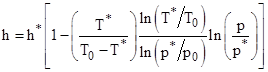
This gives the precise value of g = 32.17277 ft/sec² we selected previously, which happens to be very close to the standard value that is often used for the surface of the Earth, but for consistency under the stated conditions we must simply define g by this relation. With this, the expressions relating altitude h and pressure p below the tropopause boundary can be written as

Likewise the equation applicable above the tropopause boundary can be written as

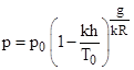
To find the pressure density (below the tropopause boundary), we start with the inverse of (6), which gives the pressure altitude as a function of the altitude

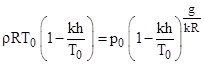
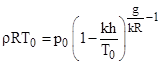
Recall from equation (2) that p = ρRT, and we also have T = T₀ – kh, so we can substitute for p to give the relation

Thus, dividing through by the quantity in parentheses on the left, we have

Solving for h, we arrive at the so-called density altitude (for the range below the tropopause boundary)

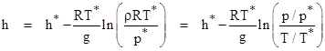
The expression for the density altitude above the tropopause boundary can be derived similarly, leading to the result

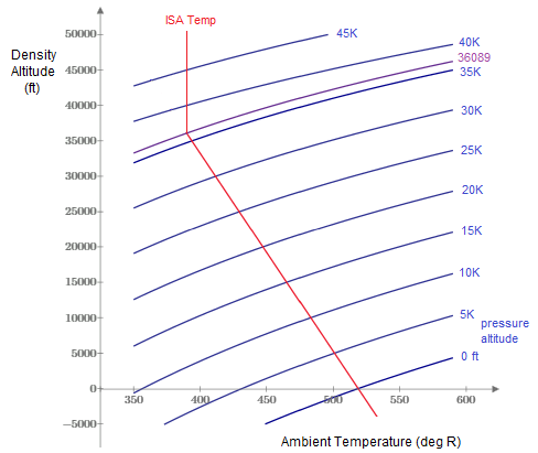
A plot of density altitude versus temperature with lines of constant pressure altitude is shown below.

The pressure altitude given by (6) equals the density altitude given by (10) on the ISA standard day temperature profile. Setting those two expressions for h equal to each other, we find that

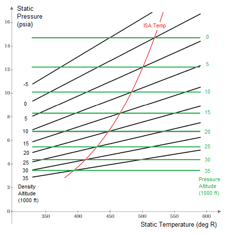
Solving equations (6) and (10) for pressure as a function of temperature and either pressure altitude or density altitude, we can plot lines of constant altitude as shown in the figure below.

So far we have assumed that the acceleration of gravity was constant over the range of interest, but in fact there is a slight reduction in g as we go up in altitude. This can be significant when dealing with the energy of an object, especially if we need to know very precisely its position as a function of actual energy. For this purpose, people sometimes use "geopotential altitude". The potential energy required to move a mass m from sea level to the geometric altitude Z is

where r_e is the radius of the Earth. Now, the acceleration of gravity, g, is a function of the distance r from the Earth's center, so if we let r_e denote the radius of the Earth (sea level, neglecting non-spherical effects), we have r = r_e + z, and so

where M is the mass of the Earth and G is Newton's gravitational constant. The force required to raise the object is F(z) = g(z)m, so we can substitute this into (11) and integrate to give

By definition, the geopotential altitude is

Substituting for the potential energy and the acceleration of gravity at the Earth's surface, and simplifying, gives the geopotential altitude as a function of the geometric altitude

Since dh/dz = r_e²/(r_e + z)² = g/g(0), it also follows that the hydrostatic equation (1) can be wrtten as dρ/dh = −ρg(0).

Return to MathPages Main Menu