Color Space, Physical Space, and Fourier Transforms

The energy distribution as a function of frequency (i.e., the power spectral density) of a beam of light can be regarded as an infinite-dimensional vector, specified by the values of the density at each of infinitely many frequencies. In other words, we can associate the spectrum of any beam of light with a unique point in an infinite-dimensional space. However, from the standpoint of human vision, the space of visible light sensations is only three-dimensional, meaning that the visual perception of any beam of light can be characterized by just three numbers. One possible basis for characterizing a beam of light consists of the intensities of a matching combination of three primary colors (e.g., red, green, blue). Another possible basis consists of hue, saturation, and intensity. Regardless of which basis we choose, the space of visual sensation has just three dimensions, rather than infinitely many.

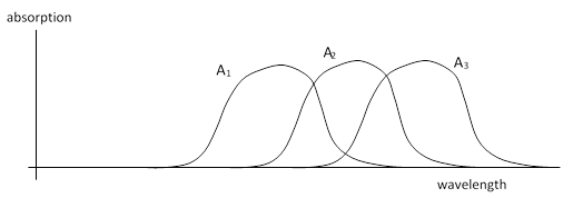
The reason our optical sensations have only three dimensions is that our eyes contain just three kinds of cones, each with a characteristic absorption spectrum. (This is discussed in more detail in Pitch and Color Recognition.) Let A₁(λ), A₂(λ), and A₃(λ) denote three linearly independent absorption spectra (meaning none of them can be expressed as a linear combination of the other two), as shown below.

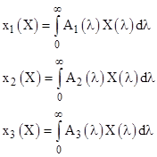
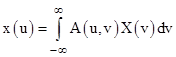
We can characterize the sensation corresponding to a beam of light with the power spectral density X(λ) by the three integrals

Thus each spectral density function X maps to a point in three dimensional space with the coordinates x₁(X), x₂(X), x₃(X). Clearly for any two spectral density functions X(λ), Y(λ) and constants α, β we have

so the mapping between spectral density functions and points in space is linear. For example, the spectral density function (X+Y)/2 maps to the point half way between x(X) and x(Y).

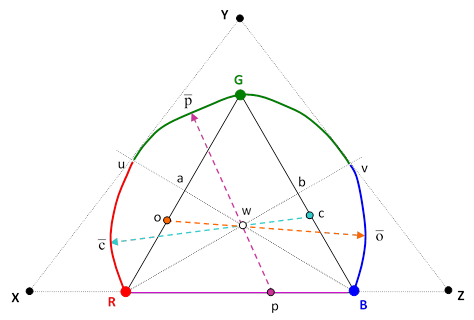
Each direction in space in the positive octant corresponds to a color sensation, and the distance from the origin signifies the intensity. (Of course, each color sensation maps to infinitely many distinct spectral density functions, due to metamerism.) If we disregard the intensity of light, and consider only the color (i.e., the hue and saturation) then the space of optical sensations can be represented on the projective plane. Every point on the projective plane can be expressed as a linear combination of any three non-colinear points. These are called barycentric coordinates. For example, we might choose as our three reference points the color sensations given by monochromatic red, green, and blue light, with the wavelengths 700, 550, and 400 respectively. Placing these at the vertices of an equilateral triangle, we can then assign mixtures of any two of these colors to the appropriate points on the lines connecting those two points, as shown below.

For any mixture “o” of R and G along the segment Ra, we can determine the amount and frequency of monochromatic light that yields the sensation of white when combined with the mixture o. This enables us to map all the monochromatic points from B to v. In the same way we can identify all the monochromatic complements of the mixtures “p” on the segment RB, and this gives the mapping of the spectral points that form the curve from v to u. Lastly we determine the monochromatic complements of the mixtures “c” on the segment Bb to give the locus of pure spectral points along the curve from u to R.

Physically every color sensation discernable to the human eye can be produced by some combination of positive amounts of the pure spectral colors, i.e., the monochromatic lights corresponding to the curved locus RuGvB. Hence the space of visible color sensations consists of the points of the convex region inside that locus (and above the line RB of purple mixtures). Each of those points can be expressed as a linear combination of our “primary” points R,G,B, but only if we allow negative contributions. For example, to match the color sensation corresponding to the pure spectral point “v” we must first mix positive amounts of G and B to give the mixture “b”, but then we must add a negative amount of R to reach the point “v”. Another way of saying this is that we must add a positive amount of R to the point “v” in order to be able to match the result with a combination of G and B.

If we want all the visible color sensations to be expressible as a positive combination of our three “primary” sensations, we need to choose three points outside the region of visible light. Essentially we want a triangle that circumscribes the entire convex region of color sensations. One such set of primaries consists of the points X,Y,Z shown in the figure above. These points do not correspond to any actual optical sensations, because they could be produced only by mixtures of pure spectral light that contained some negative contributions, and there is (as far as we know) nothing in nature corresponding to light of negative energy. Nevertheless, these “imaginary” primaries are convenient because every actual color sensation can be expressed as a positive combination.

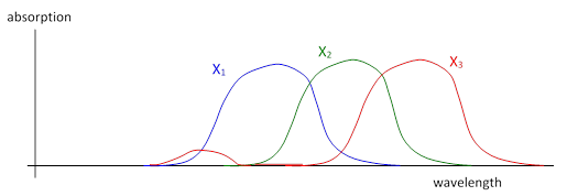
One interesting aspect of our sense of color is that although red is normally associated with the low end of the range of visible frequencies, the color violet (at the high end of the frequency range) has a reddish-blue appearance. This is because the predominantly low-frequency cones in our eyes also have some absorption at the very high frequencies. Thus the actual absorption spectra of our optical senses are somewhat as shown below.

This wrap-around effect may be due to the “octave effect”, because the longest visible wavelengths are about 760 nm (extreme red) and the shortest are about 380 nm (extreme blue), which is a ratio of exactly 2 to 1. Thus the first harmonic of the extreme red absorption cones is in the extreme blue frequency range, so it isn’t surprising that the red cones resonate slightly in response to violet light.

This suggests an interesting mechanism for non-local effects in metric spaces. It’s possible for a pure monochromatic light near the blue end of the spectrum to be somewhat reddish. When we say this we are employing two different meanings of “red”, one being a particular frequency, which is strictly at the low end of the visible frequencies, and the other being the sensation arising from stimulation of the “red” cones in our retinas, which actually have some degree of sensitivity at all frequencies.

In discrete terms, we can consider a system with an N-dimensional phase space with coordinates X₁, X₂, …, X_N, and a linear projection into a reduced phase space of M ≤ N dimensions with coordinates x₁, x₂, …, x_M. For example, with N = 5 and M = 2 we have

where the coefficients A_ij are constants. Clearly there are three degrees of metamerism in this mapping, because for any given coordinates x₁,x₂ we can freely choose any three of the X coordinates and still solve for the remaining two. If we change from discrete to continuous indices, letting u denote the indices on x, and v the indices on X, then this transformation becomes something like

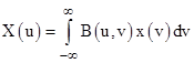
but we apparently lose the distinction between the dimensionalities of x and X. In the discrete case, with M = N, the transformation from X to x is invertible, provided the A matrix has an inverse, i.e., provided the rows of A are linearly independent. In the continuous case we could seek a two-dimensional function B(u,v) such that

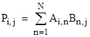
In the discrete case the product P = AB of two square arrays A and B is

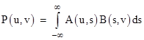
and we can define the analagous “product” of two continuous functions A(u,v) and B(u,v) as

Analagous to the diagonal identity matrix, we can also define the “identity” function as δ(u–v) where δ(t) is the Dirac delta function, and then two functions A and B would be considered inverses of each other if and only if their product is the identity function.

If the two-dimensional function A(u,v) is to be invertible, the set of one-dimensional functions A(k,v) for all constants k must be linearly independent. This rules out a large class of functions. For example, the function uv is not invertible, because each function kv is just a scaled version of v. Likewise the function uv + u²v² is not invertible, because there are only two linearly independent functions of the form kv + k²v². In other words, given two functions a₁v + b₁v² and a₂v + b₂v² we can express any other function of the form a₃v + b₃v² as a linear combination

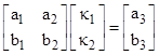
by solving the simultaneous equations

for the constants κ₁ and κ₂. By the same token, any other finite polynomial in u and v cannot be invertible. However, this reasoning shows that an infinite polynomial could be invertible. The most natural choice is the exponential function

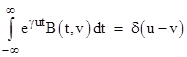
for some constant γ. Each of the functions e^γkv for constant k is linearly independent of all the others. Setting A(u,v) equal to this exponential, we seek the “inverse” function B(u,v), i.e., the function such that

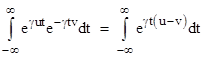
Notice that if we set B(u,v) equal to the algebraic inverse of e^γuv, namely e^–γuv, the above integral is

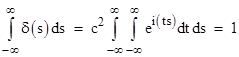
We can make this integral vanish for all non-zero values of u – v by setting γ = i, because in this case the integrand simply traces a unit circle about the origin uniformly as a function of t, and each cycle integrates to zero, and the peaks diminish in magnitude. On the other hand, if u – v equals exactly zero, the integrand is unity, so the integral is infinite, just as required for the delta function. The only remaining requirement is for the integral of the delta function to equal unity. We expect it will be necessary to scale the functions A(u,v) and B(u,v) by some constant factor c, defined such that

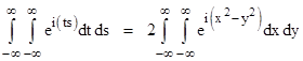
If we define two new variables s = x – y and t = x + y we have ts = (x² – y²), and the Jacobian of the transformation is

which implies (ds)(dt) = 2(dx)(dy). Also, the limits of integration are the same, so the double integral in the previous expression can be written as

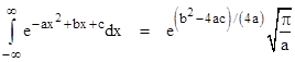
Now we recall from a previous note the integral

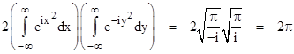
so if we split the integrand of our double integral and evaluate each part separately we get

Therefore, the normalizing factor is

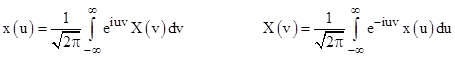
Thus we have the reciprocal transformations

We recognize these as Fourier transformations. It’s interesting how naturally they arise from the basic requirements for an invertible continuous transformation, following closely the analogy with discrete matrices.

Return to MathPages Main Menu