Fourier Transforms and Uncertainty Relations

The function exp(–x²) has no simple closed-form indefinite integral, but the related function x exp(–x²) does have a simple integral, namely,

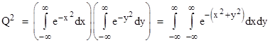
This identity can be used to evaluate the definite integral of exp(–x²) from x = –∞ to +∞. Letting Q denote the value of this definite integral, we can write

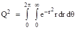
In terms of polar coordinates on the x,y plane we have x = r cos(θ) and y = r sin(θ), and therefore x² + y² = r². The Jacobian of the transformation is

so the incremental area element is

Hence the double integral expressed in terms of r,θ coordinates is

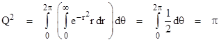
Making use of equation (1) to evaluate the interior definite integral, we have

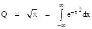
Therefore the definite integral of exp(-x²) from –∞ to ∞ is

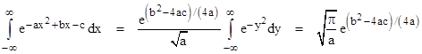
More generally, if we replace the exponent  –x²  with  –ax² + bx – c,  we can define the parameter

in terms of which we can write

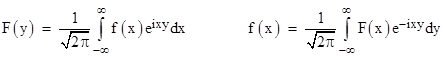
This definite integral is particularly useful when considering the Fourier transform of a normal density distribution. Recall that for any function f(x) we can define another function F(y) that satisfies the relations

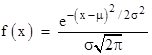
These two functions are a Fourier transform pair, i.e., each of them is the Fourier transform of the other. Now, if f(x) is the normal probability density function

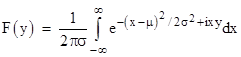
then the Fourier transform is

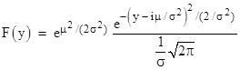
so the exponent in the integral is of the form -ax² + bx + c with a = 1/2σ², b = iy + μ/σ², and c = –μ²/(2σ²). Hence the Fourier transform of the normal density distribution is

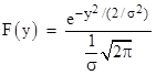
Choosing our scales so that the mean of f is zero, i.e., so that μ = 0, the above expression reduces to

In other words, the Fourier transform of the normal distribution with mean zero and standard deviation σ is also a normal distribution with mean zero, but with standard deviation 1/σ. This shows that the variances of the f and F distributions satisfy the "uncertainty relation" var(f) var(F) = 1. This equality is the limiting case of a general inequality on the product of variances of Fourier transform pairs. In general, if f is an arbitrary probability density distribution and F is its Fourier transform, then

Notice that f and F are just two different ways of characterizing the same distribution, one in the amplitude domain and the other in the frequency domain. Given either of these distributions, the other is completely determined.

The relation between conjugate variables (such as position and momentum) in quantum mechanics can be expressed in terms of the relation between Fourier transform pairs. Consider a physical system with just one degree of freedom, represented by the operator q, and let p denote the operator for the corresponding momentum (i.e., the generalized momentum of q in the usual Hamiltonian formulation). The basic commutation relation between these operators is

Notice the symmetry between the p and q operators if we replace i with –i. The usual Schrodinger representation of this system takes the observable q as a "diagonal" operator, i.e., with the eigenvalues specified explicitly, and then the corresponding momentum operator is defined as

However, we could (in theory) just as well take p as a diagonal operator, and then q would be given by

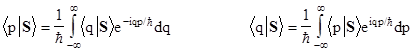
Dirac referred to this as the momentum representation of the system. This again shows the symmetry between q and p under an exchange of i and –i. Indeed if we let <q|S> and <p|S> for any given state S denote the probability amplitudes that measurements corresponding to the operators q and p will return the eigenvalues q and p respectively, then we find

In other words, the probability amplitude distributions of two conjugate variables are simply the (suitably scaled) Fourier transforms of each other. We saw previously that the dispersions (variances) of two density distributions that comprise a Fourier transform pair satisfy the inequality (2), so the variances of the probability amplitude distributions of conjugate observables in quantum mechanics satisfy such an inequality. Thus Heisenberg's uncertainty principle for conjugate pairs of observables follows directly from the fact that those observables are essentially the Fourier transforms of each other.

Of course, this attribute of Fourier transform pairs is purely mathematical, and has no a priori applicability to pairs of observables such as position and momentum, or time and energy. The physical content of quantum mechanics is based on the two relations

where E is energy, p is momentum (in one dimension),  is Planck's (reduced) constant, ω is the frequency with units second^–1, and k is the wave number with units meter^–1. These relations were introduced in the early 1900's by Planck, Einstein, and deBroglie to account for non-classical phenomena such as cavity radiation and the photo-electric effect, both of which depend on the particle-like behavior of entities that had previously been modeled as waves, as well as phenomena involving wave-like behavior of material particles. These are the relations that associate the familiar observables of energy, momentum, space, and time, with the frequency domain. Indeed in terms of the characteristic time τ = 1/ω and distance  = 1/k the above relations can be written as

which already clearly reveals the conjugacy of time and energy, and of distance and momentum. In view of this, it isn't surprising to find that the product of the dispersions of two conjugate observables (such as position and momentum) cannot be less than one quanta of action, represented by .

In a sense, there is also a conjugacy between space and time - two observable that had been regarded as disjoint and independent prior to the early 1900s. In special relativity the inertial space and time intervals dx and dt between two events are components of a single invariant spacetime interval ds between those events. These intervals are related according to the Minkowski metric, which can be written in the form

This can be regarded as an "uncertainty relation" for space and time. In general, physics was based, prior to 1900, on the premise that  and 1/c² were both zero. With the advent of quantum mechanics and special relativity, it was realized that they both have non-zero values, although they are extremely small in terms of ordinary units.

Return to MathPages Main Menu