The Electric and Magnetic Fields of a Moving Charge

The electric and magnetic fields E and B at point R and time t due to a particle of charge q with the worldline R_q(τ) can be derived from the retarded potentials

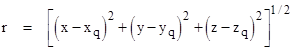
where

For convenience we also define the unit vector

The electric field E is given in terms of the potentials by

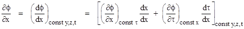
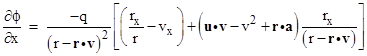
The scalar potential ϕ is explicitly a function of the coordinates x, y, z, and t of the field point (R,t), but also implicitly as a function of the retarded time τ, which (for a given charge worldline) is itself a function of the field point coordinates. Thus the partial derivative of ϕ with respect to x at constant y,z,t must account for the implicit dependency as follows

So, we have the partial

We can easily verify that the partial derivatives on the right hand side are

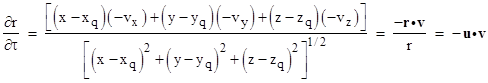
For example, since

we have

The other partial derivatives can be derived similarly. Also, since t – τ = r, we have for constant  t  the relation

which we can solve for the total derivative of τ with respect to x to give

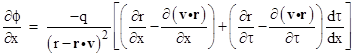
Making these substitutions into the expression for ∂ϕ/∂x we get

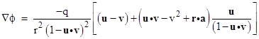
Combining this with the corresponding expressions for ∂ϕ/∂y and ∂ϕ/∂z gives the gradient

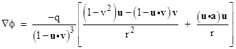
Re-arranging terms, this can be written as

If this were the complete electric field, we see that the first term would give the “electrostatic” component proportional to 1/r², and the second term would give a “radiation” component proportional to 1/r due to acceleration of the charge. For example, if the charge was oscillating in a small range on the x axis, the x component of the gradient also oscillates, and the wave of oscillations propagates outward along the x axis at the speed of light. (This is discussed in more detail in The Electric Potential of a Moving Charge.) However, this is a longitudinal wave, i.e., the oscillating gradient vector is parallel to the direction of propagation of the wave. Furthermore, the maximum intensity is along the axis of the oscillating charge, and drops to zero in the perpendicular plane. These characteristics are contrary to what we know about propagating disturbances in the electric (and magnetic) fields, in which the field vector oscillations are are transverse to the direction of propagation of the waves, and which vanish along the axis of an oscillating charge.

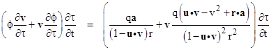
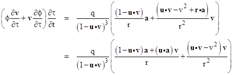
In order to determine the actual behavior of the electric field due to a moving charge we must take into account the term ∂A/∂t, which can also be written in terms of ϕ and v as

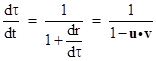
To determine dτ/dt we differentiate the relation t – τ = r with respect to t and write the result in the form

Solving this for dτ/dt gives

Substituting into the previous expression and re-arranging terms gives

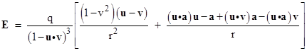
Subtracting this from the negative gradient of f gives the total electric field

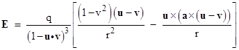
Making use of the vector triple-product identity

to simplify the numerator of the second term inside the brackets, we get

Naturally if the velocity and acceleration of the charge are both zero, this reduces to Coulomb’s law E = qu/r².  Thus the force QE on a test charge Q at the field point R will be in the positive u direction (i.e., pointing from q to Q) if Q and q have the same sign, and this represents a repulsive force on Q.  If q and Q have opposite signs, the force on Q is in the negative u direction, representing an attractive force, i.e., a force toward q.

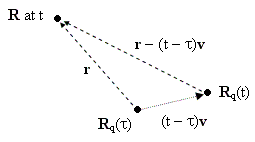
If the acceleration is zero but the velocity is non-zero, the electric field points either positively or negatively along the direction of u – v, which may seem surprising at first, because we know the electric field of a uniformly moving charge points directly toward (or away from) the instantaneous position of the source charge with respect to any system of inertial coordinates. However, this is actually consistent with our result, because u is the unit vector pointing from the past position of the charge to the present field point, as illustrated below.

Thus the vector from the charge at time t to the field point at t is r – (t – τ)v. Dividing this by r = t – τ gives u – v, which confirms that the electric field at R points along the direction from R to the present (not the retarded) position of the charge.  It’s also worth noting that the magnitude of v is always less than the magnitude of the unit vector u (because we have taken units of space and time such that c = 1), so the sign of the electric field (with a = 0) is always positive for any velocity v, positive or negative.

If we consider one-dimensional motion and field points along the axis of motion, then the second term (the one involving acceleration) drops out (because the acceleration, velocity, and displacement vectors are all parallel), the unit vector u becomes 1 and the velocity along the axis of motion is the scalar v, and the equation for the electric field reduces to

As always, v represents the velocity of the charge at the prior time τ, and r is the present position of the field point relative to the charge’s position at the prior time τ.  It follows that the effect on the field of a change in the speed of the charge propagates away from the charge at the speed of light. However, for the reason noted above, this ripple effect cannot cause the sign of E to change, so this isn’t true “radiation”.

In full generality, with arbitrary positions, velocities, and accelerations, the second term in the brackets in the expression for E is non-zero (provided v does not equal u). This term can be either positive or negative, depending on the sign of the acceleration. The magnitude of the second term drops off in proportion to 1/r, as opposed to 1/r² for the first term. Of course, the acceleration a is at the prior time τ, so the effect of any acceleration propagates away from the charge at the speed of light. Also, the direction of this term is perpendicular to the unit vector u from the retarded position of the charge, confirming our expectation that the radiative component of the electric field is transverse to the direction of propagation.

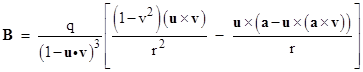
By a derivation similar to the one above, it can be shown that the magnetic field of the moving charge is

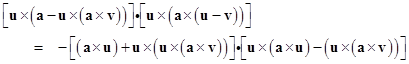
This shows that the radiation component of the magnetic field is also perpendicular to the unit vector u from the retarded position of the charge, so it too (like the electric component of radiation) is transverse to the direction of propagation. Furthermore, notice that the dot product of the electric and magnetic radiation components (multiplied by r²) is

where we have made use of the fact that u x a = - a x u.  Setting m = a x u and n = u x (a x v), this dot product can be written as the negative of

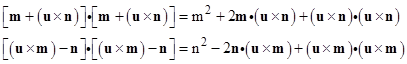
The first and last terms on the right side are obviously zero, because u x m is perpendicular to m, and u x n is perpendicular to n. Therefore the dot product is

The first and last terms on the right side cancel out, and both factors of the middle term are zero because m and n are both perpendicular to u. Hence the dot product vanishes identically, signifying that the radiation components of the electric and magnetic fields are perpendicular to each other (as well as both being perpendicular to u).

It’s also worth noting that the radiation components of the electric and magnetic fields are equal in magnitude. To prove this, determine the squared magnitudes by taking the dot product of each vector with itself. This gives the two quantities

Since m and n are each perpendicular to u, the middle terms of both the above expressions vanish. Also, the last terms of the two expressions can be expanded to the form

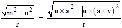
Again, since m and n are perpendicular to u, the last terms vanish, so the magnitudes of the electric and magnetic radiation components are both equal to

Since the radiation component of B is equal in magnitude to the radiation component of E, and perpendicular to both E and u, we have B_rad = u x E_rad.

Return to MathPages Main Menu