The Electric Potential of a Moving Charge

The electric field vector E at a given time and place is defined as the force per unit charge that would be exerted on a stationary charged particle at that time and place. Thus the force on a stationary charge q subject to the electric field E is f = qE. If the charge q is not stationary, but moving with velocity v, we find in general that it experiences an additional force whose magnitude and direction in a given physical setting varies with v in such a way that the total force is f = qE + qv x B where B is called the magnetic field vector.

It is possible and convenient to define a scalar field ϕ(x,y,z,t) and a vector field A(x,y,z,t) such that

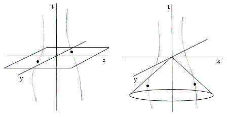
The fields ϕ and A are also called the electric and magnetic potentials, respectively, and c is the speed of light in vacuum. Historically, the original expressions for the electric potential (as proposed by Weber, Neumann, and others) were based on the model of Newtonian gravity, so the potential was assumed to be inversely proportional to the radial distance from the source charge. The the potential at the origin of an inertial coordinate system contributed by a charge q at position r was assumed to be of the form q/|r|. It was also assumed that, as with Newtonian gravity, the potential due to a charge acted instantaneously at all distances. This conception of electric potential changed in the 1880’s when Ludwig Lorenz suggested that the potential at the origin at time t should be due to all the charges not on the instantaneous time slice of the origin, but on the past light cone of the origin, as illustrated below.

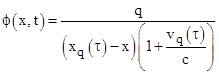
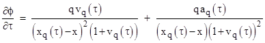
One consequence of the retardation is that the intensity of the potential becomes a function not just of the spatial distance but also of the speed of the source charge. A charge approaching the origin spends more time on the past light cone of the origin than it would if it was moving parallel to or away from the origin. (This is discussed in greater detail in the note on Retarded and Advanced Potential.) It can be shown that the electric potential at location x and time t due to a charge q moving along the x axis at the location x_q (assumed to be greater than x) and moving with the velocity v_q when it intersects the past light cone of (x,t) is

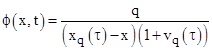
where τ is the time when the charge passed through the past lightcone of (x,t), which implies that t - τ = [x_q(τ) – x]/c.  If the propagation speed c were infinite, this would reduce to ϕ(x,t) = q/(x_q-x) at any time t and the gradient in the x direction would be simply ∂ϕ/∂x = q/x², signifying a purely Newtonian inverse-square force law (noting that f_x = –∂ϕ/∂x). However, if c is finite, we can chose units such that c = 1, and the potential can be written as

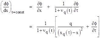
where t - τ = x_q(τ) – x. The partial derivative of ϕ with respect to x is given by taking the total derivative of ϕ with respect to x at constant t. In this case, τ varies as a function of x, even at constant t, and therefore so do x_q(τ) and v_q(τ).  With this in mind, we see that the total differential of ϕ (at constant t) can be expressed as

Dividing through by dx gives

Differentiating the relation t - τ = x_q(τ) – x with respect to τ at constant t gives

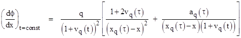
so we have

The first term in the square brackets represents the Newtonian inverse-square component, but what about the second term?  The partial derivative of ϕ with respect to τ is

Inserting this into the previous expression, we arrive at the complete gradient of the potential with respect to x:

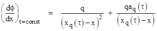
If the velocity v_q of the charge is only a very small fraction of the speed of light, it is negligible compared to 1, and the above expression reduces to

Again, the first term represents a force pointing in the direction of the charge (for an oppositely-charged test particle) and with a magnitude that drops off in proportion to the inverse-square of the distance, but the second term represents something quite different.  It is a force proportional to the acceleration of the charge, so it can be positive or negative, and the magnitude drops off as the inverse distance (not the inverse of the squared distance). Furthermore, the force at the coordinates (x,t) depends on the acceleration of the charge at the earlier time τ, which implies that the effect of the acceleration propagates outward from the charge at the speed c.

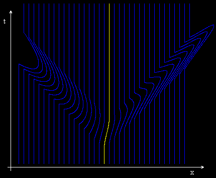
Since the potential is essentially proportional to the inverse of the distance, it might seem counter-intuitive at first that there is a component of the derivative that drops off as the inverse distance, but this component is due to the scaling effect of the retarded velocity-dependent factor in the expression for the potential. With this extra factor, the product rule of differentiation automatically results in two terms, one of which is inversely proportional to the square of the distance, and the other of which is inversely proportional to the first power of the distance. This is illustrated pictorially in the figure below, showing lines of constant electric potential on the x axis near a charged particle that is initially stationary, then accelerates in the positive x direction, and then slows to a stop again.

The yellow line is the worldline of the charged particle, and the blue lines are lines of constant electric potential. The acceleration of the charge results in a “bunching together” of the lines of potential by a factor proportional to the distance from the charge, so this offsets one of the distance factors in the denominator. The drawing also shows how, in the latter part of the wave, the derivative changes sign. For example, the right-most line of potential actually lies directly to the left of the neighboring line on the latter part of the wave. (This drawing also illustrates that the electrostatic force exerted by a charged particle on a test particle at a distance D does not change until a time D/c after the source charge moves.)

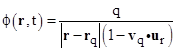
We can deduce additional information about the structure of electromagnetic waves by examining the lines of constant potential in the xy plane. To do this we can begin with the generalize expression for the retarded scalar potential (called the Lenard-Weichert potential)

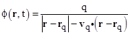
where u_r is a unit vector in the direction of r – r_q.  Since ur = (r-r_q)/|r-r_q|, we can multiply through by the scalar |r-r_q| to give

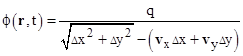
If we consider just the plane z = 0 we can write this in terms of the x and y increments between the charge and the field point as

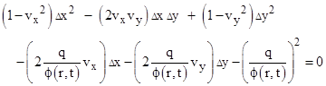
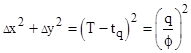
where v_x and v_y are the x and y components of v_q. Re-arranging terms to isolate the radical and then squaring gives the conic

(On the Δy = 0 plan this reduces to our previous one-dimensional formula.) Also, on the time slice t = T we have

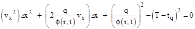
The charge q in our example has no velocity in the y direction, so we can substitute v_y = 0 into the prior conic equation to give the quadratic

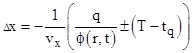
Solving this for Δx gives

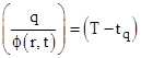
So, given the charge q and the position x_q(t_q) and speed v_q(t_q) = v_x(t_q) of the electron as functions of time, we can choose a time-slice T and a potential ϕ, and then for every value of t_q we can determine the locus of x,y points on the time slice T with potential ϕ. To do this, for any given t_q, we first check to see if v_x(t_q) is zero. If it is, then the quadratic is satisfied if and only if

If this equality does not hold, then the time tq does not contribute a potential of q to any point on the timeslice T. On the other hand, if this equality does hold, then the locus of points is the circle

If v_x(t_q) is not zero, then we compute Dx from the quadratic solution (assuming the roots are real), and then Δy from the above equation. In any of these cases, once we have found a solution (Δx, Δy) we compute the actual coordinates

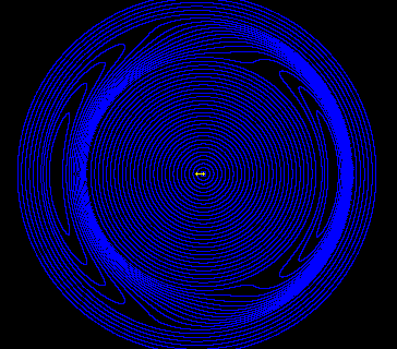
Carrying out this procedure for the same moving charge as in our previous example, we can generate a plot of the lines of constant scalar potential shown below for the time slice T = 16.

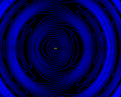
The outer circular loci represent the lowest potential, generated by the charge when it was futhest in the past, at the x value of the left-most end of the yellow projected path, which is the center of the outer circles. The inner circles are the greatest potential, centered around the right-most end of the yellow path, i.e., the final position of the charge. The transitional region is the potential corresponding to the period of acceleration and motion of the charge. In this example the charge undergoes only one cycle of acceleration, so there is just a single set of equi-potential “packets” emanating in both directions, but with multiple accelerations there would be a series of nested packets, propagating outward at the speed c.  This is illustrated in the figure below, which shows lines of constant f in the xy plane for the near field of a charged particle moving sinusoidally on the yellow range of the x axis.

The preceding examples all consisted of a single moving charged particle, but most electromagnetic waves in nature are produced by dipole oscillations, or by oscillations of systems that can be closely approximated as dipoles. The contributions to the potential of the two charges of a dipole tend to cancel each other out along the axis of a dipole.

Return to MathPages Main Menu