Laminar Transformations

A linear transformation is called laminar if it is of the form I + Q where I is the identity transformation and Q is any matrix whose square is the null matrix. For any laminar transformation we have

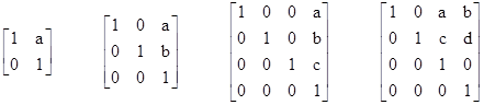
Some examples of laminar transformations are shown below.

where a,b,c,d are constants. Obviously any permutations of the row/columns also give laminar transformations. The examples above are each maximal in the sense that if all the lettered elements are non-zero, then none of the zero elements could be changed to a non-zero value without destroying the laminarity of the transformation. Note that there are maximal laminar 4th-order transformations with three degrees of freedom, and others with four degrees of freedom. In general there are maximal laminar kth-order transformations with rs degrees of freedom for every pair of positive integers r,s such that r + s = k. Each of these represents an equivalence class consisting of all the transformations of that form. Allowing for the possibility that some of the lettered elements may be zero, it’s possible for a given transformation to be in more than one equivalence class, so this equivalence relation is not transitive.

It’s possible to express general linear transformations as compositions of laminar transformations. For example, consider the two-dimensional plane with Cartesian coordinates x,y, and the two laminar transformations x′ = x + qy, y′ = y and x″ = x, y″ = y − qx. In matrix form these are written as

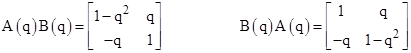
Letting A(q) and B(q) denote the coefficient matrices of the left and right hand equations respectively, the compositions of these two transformations are

Hence these transformations are not commutative, and neither of them is symmetrical in x and y. Making use of the linearity of laminar matrices, the first of these equations can be written in the equivalent form

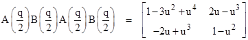
Now, to create a transformation that is more nearly symmetrical between A and B (and therefore between x and y), consider the transformation consisting of those same factors but interleaved in alternating order, as shown below.

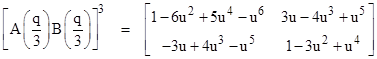
In this expression we have put u = q/2. In the same way we can interleave n copies of A(q/n)B(q/n) for any given n. With n = 3 we get

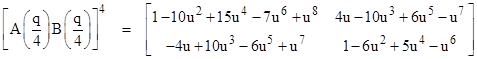
where u = q/3. With n = 4 we get

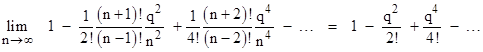
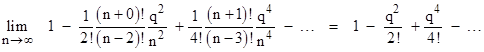
where u = q/4. Clearly the terms of the composite matrix are polynomials in q/n with coefficients given by diagonal slices of Pascal’s triangle with alternating signs. (See Linear Fractional Transformations for the roots of these polynomials.)  In the limit as n goes to infinity (so we are interleaving infinitely many infinitesimally small laminar transformations), the upper left diagonal term approaches

We recognize this as the series expansion of the cosine of q. The lower right diagonal term approaches the same function, as shown by

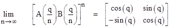
Likewise the off-diagonal terms both approach the sine of q, so we have

which is the Euclidean rotation transformation for a clockwise rotation about the origin through the angle q. Thus we can regard rotation in the plane as being composed of a continuous alternating mixture of infinitesimal laminar transformations. Varying the mixtures would lead to other transformations.

Another simple example of a laminar transformation in physics is the Galilean transformation in one space dimension and one time dimension, which has the form

Strictly speaking, a Galilean transformation in physics relates two systems of (putative) inertial coordinates with mutual velocity v, but for our purposes we will use the term to refer to any coordinate transformation that consists of an off-setting of the space coordinates as a linear function of the time coordinate. Thus neither x,t nor x′,t′ need be inertial coordinate systems and v need not be the speed between them. Any such transformation can be written in matrix form as

The transpose of this transformation gives a linear off-setting of the time coordinates as a linear function of the spatial coordinate, and can be written as

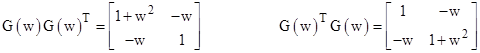
Letting G(w) denote the coefficient matrix of the formal Galilean transformation with arbitrary parameter w, the linearity of these laminar matrices is expressed by G(a)G(b) = G(a+b). The compositions of G(w) and G(w)^T are

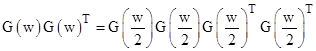
Neither of these is symmetrical in x and t, because the diagonal terms are not equal. However, the asymmetry is only of the second order.  Just as in the previous case, we can make use of the linearity of laminar matrices to write the first of these equations in the equivalent form

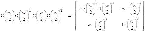
Interleaving the terms on the right side gives

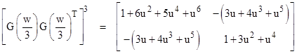
where u = w/2. Likewise way we can interleave n copies of G(w/n)G(w/n)^T for any given n. With n = 3 we get

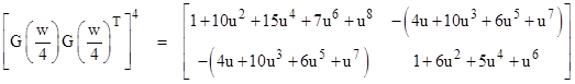
where u = w/3. With n = 4 we get

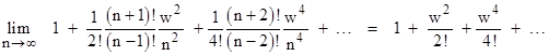
where u = w/4. Again the terms of the composite matrix are polynomials in w/n with coefficients given by diagonal slices of Pascal’s triangle, but this time without alternating signs. In the limit as n goes to infinity (so that we are interleaving infinitely many infinitesimally small laminar transformations), the upper left diagonal term approaches

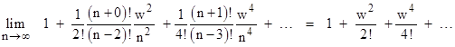
We recognize this as the series expansion of the hyperbolic cosine of w. The lower right diagonal term approaches the same function, as shown by

Likewise the off-diagonal terms both approach the hyperbolic sine of w, so we have

In order for a particle moving with speed v in the positive x direction to be stationary in terms of the transformed coordinates, the ratio of the upper right term to the upper left term must be –v. Hence we have

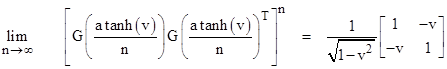
Therefore, w = atanh(v), and we can insert this into the previous expression to give

which is the Lorentz transformation. (The limit is the same if we transpose G and G^T on the left hand side of this expression.)

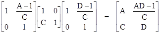
The preceding discussion focused on producing symmetric expressions, which required going over to the limit of an infinite sequence of transformations, but it’s also possible to expression Euclidean and Lorentz transformations (for example) using finite products of laminar transformations, although not symmetrically. Of course, the determinant of any laminar transformation is 1, so the product of any number of such transformations must have a determinant of 1, but any transformation that satisfies this condition can be expressed as the product of laminar transformations. For order 2, no more than three laminar transformations are required, as shown by the identity

Letting B denote the upper-right element of the right hand matrix, we have AD – BC = 1 as required. If the target matrix has special symmetries we can specialize this result. For example, a Euclidean rotation in two dimensions through an angle θ can be expressed in either of the forms

where

Thus a Euclidean rotation can be expressed as the composition of a laminar shift of the x coordinates followed by a laminar shift of the y coordinates followed by another laminar shift of the x coordinates, or conversely by laminar shifts of the y, x, and y coordinates. Likewise a Lorentzian boost through a speed v in one space dimension and one time dimension can be expressed in either of the forms (1) with

Thus a Lorentz boost can be expressed as two Galilean transformations and one laminar temporal transformation, or equivalently as two laminar temporal transformations and one Galilean transformation. Notice that for small v (which is to say, for velocities that are small compared with the speed of light) we have α ≈ −v/2 and β ≈ −v, and the combined transformations are nearly commutative.

Of course, what we have referred to as “Galilean transformations” in these expressions are not the same as the classical Galilean transformations for the overall change from one (putative) inertial coordinate system to another, because the parameter in these formal transformations is not the mutual speed v between the two systems of coordinates. The physical content of the Lorentz transformation is essentially encoded in the denominators of the expressions for α and β, which we chose so that the compositions would give the Lorentz transformation. If we didn’t know what the correct Lorentz transformation was to begin with, we would not have known what expressions to use for α and β. In contrast, the prior discussion involving symmetrical infinitesimal laminar transformations arrived at the expressions for Euclidean and Lorentz transformations purely by imposing symmetry on the two coordinates, without relying on prior knowledge of the correct expressions.

As an amusing aside, the fact that non-laminar transformations can be expressed as mixed products of laminar transformations is sometimes invoked by pseudo-scientific crackpots as “proof” that relativistic time dilation is impossible. It’s true that, since the diagonal components of a laminar transformation (such as a Galilean transformation or its transpose) are unity by definition, the time-time coefficient is unity, and hence there is no time dilation, as is easily seen by applying such a transformation to the interval from t = 0, x = 0 to t = 1, x = v, and noting that the return interval has the same elapsed transformed time by symmetry. However, the time-time coefficient of compositions of laminar transformations from different classes is not necessarily unity. A non-trivial Lorentz transformation is the product of at least three laminar transformations, and as we’ve seen, the resulting time-time coefficient of the standard transformation is the familiar factor 1/(1−v²/c²)^−1/2, which is responsible for the time dilation. Needless to say, this isn't paradoxical, because although the Lorentz transformation consists of a product of laminar factors, those factors are from different classes, and hence the composition of those transformations need not be (and is not) laminar. This is no more paradoxical than the fact that rotations about the x axis are commutative, and rotations about the y axis are commutative, but mixed rotations composed of those two kinds of rotations are not commutative.

Return to MathPages Main Menu