Linear Fractional Transformations

1 Introduction

A linear fractional transformation (LFT) is defined as a function of the form

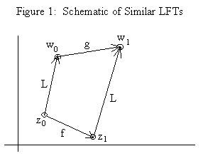
where a,b,c,d are complex constants. Every LFT defines a one-to-one mapping of the extended complex plane (C U ∞) onto itself. Two LFTs f and g are similar iff there exists a purely linear transformation L(z) = αz + β where α and β are complex constants such that

for every complex z. (The condition is reciprocal, because if L is a linear function, then so is the inverse of L.) This condition implies a mapping between the iterates of f and the iterates of g as shown schematically in Figure 1. In essence, letting z_k denote the iterates of f for any given initial value z₀, and letting w_k denote the iterates of g with the corresponding initial value w₀ = L(z₀), it follows that if f and g are similar, then w_k = L(z_k) for all k. In other words, the iterates of f can be mapped to the iterates of g by the linear function L, and since a linear transformation of the complex plane consists of (at most) a simple translation, a rotation about the origin, and a uniform scale change, it follows that the configuration of points L(z_k) is geometrically similar to the configuration of points z_k.

mob2

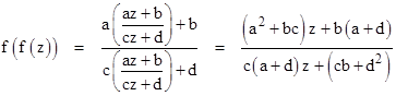
To derive necessary and sufficient conditions for similarity, suppose the two LFTs

are similar. Then by definition there exists a linear function L(z) = αz + β such that L(f(z)) = g(L(z)), so we have

Substituting for f(z) and L(z) into this equation gives

If α was zero then L would simply be a constant, and if c or C was zero the respective LFT would simply be a linear function, so we set these degenerate cases aside and consider the general case with α,C,C all non-zero. We can therefore normalize each side of the preceding equation by dividing through by c or Cα respectively (so the coefficients of z in the denominators are zero), and then equate the three remaining corresponding coefficients, which gives the three conditions

Solving the first and third conditions for α and β we get

Substituting this expression for β into the second condition and solving for α gives

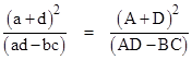
(assuming ad – bc ¹ 0). Equating this with the previous expression for α, we arrive at a necessary and sufficient condition for the LFTs f and g to be similar:

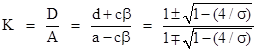
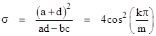
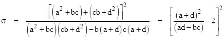
This shows that for any given LFT (az+b)/(cz+d), the similarity class is determined solely by the parameter (a+d)²/(ad–bc). Hereafter we will refer to this as the similarity parameter, and denote it by σ. Thus, for any LFT (az+b)/cz+d) we define

Two LFTs f and g are said to be conjugate if there exists an LFT h such that h(f(z)) = g(h(z)) for all z. This is identical to the definition of similarity, except that similarity requires h to be purely linear. Thus, similarity would seem to be a more restrictive condition than conjugacy. However, the necessary and sufficient condition for f and g to be conjugate is exactly the same as the condition for similarity (cf. Complex Functions, p 32, Jones and Singerman, 1987). The only strength gained by allowing h to be an LFT instead of a linear function is in the "singular" cases when the coefficients of the linear coupling function L are not well defined, such as when c, C, (a+d), or (A+D) are equal to 0. However, when (a+d) = 0 the only conjugate LFTs are those with A+D = 0. Thus, returning to the previous conditions and inserting (a+d) = (A+D) = 0, we find that in this case it is necessary and sufficient for α to be given by (1). Thus, the only case when conjugacy can exist without a well-defined linear similarity correspondence relationship between the two LFTs is if c or C equal zero. The first of the three conditions above implies that is either c or C is zero, then the other is also zero, unless α is zero, which would imply a degenerate linear function.) In these cases, by the inclusion of the "point at infinity" (which is the same expedient used to ensure closure of the LFT iterates) we can include among the linear similarity relations those with infinite coefficients (and, conversely, zero coefficients).

2 Closed Form Expressions For the nth Iterate

To find a closed-form expression for the nth iterate z_n of the linear fractional transformation f(z) = (az+b)/(cz+d), it is most convenient to consider a similar function, g, having the sequence of iterates w₀, w₁, w₂, ... where wk is related to z_k by a linear function

for some complex constants α and β. Our objective is to find a linear transformation such that a closed-form expression for w_n (the nth iterate of g) is easy to determine. In general, the original LFT can be expressed in terms of w as follows

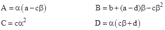
Solving for w_k+1 gives

where

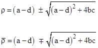
Notice that if c is not equal to zero, we cannot force C to equal zero (except by putting α = 0, which is singular). This rules out any chance of finding coefficients α,β for which w_k+1 = Kw_k. However, there are several other "nice" LFT forms for which a closed-form solution can easily be found. One such, which we will call the "bi-polar" form, is

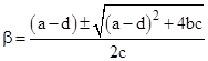
Every LFT (az+b)/(cz+d) with two distinct fixed points is similar to an LFT of this special form. The coefficients α and β of the linear similarity function are determined by setting B = 0, which implies that

We then impose the condition (C+D)/A = 1, which implies

Substituting the previous expression for β and solving for α gives

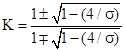
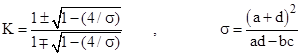
This is determined by mapping the two fixed points to the points 0 and 1 on the complex plane. We will refer to this as the bi-polar form of the given LFT similarity class. The value of K here is given by

Notice that this implies

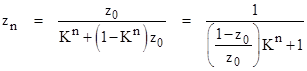
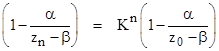
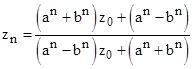
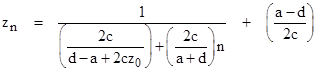
The "K form" has fixed points at 0 and 1, and it can be shown by induction that z_n has the convenient closed-form expression

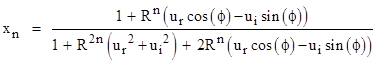
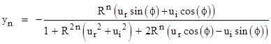
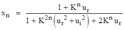
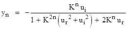
In this case the periodicity requirement is simply . It's interesting that to convert a purely real LFT to this "bi-polar K" form, the real axis is mapped to the line 0.5 + μi, which figures in the Riemann Hypothesis.

The real and imaginary components of z_n = x_n + iy_n can be expressed in closed form in terms of the components of K and z₀. If we set

then the components of z_n are given by

where f = nθ. This shows that the action of the LFT on the complex plane is entirely dependent on the magnitude and phase angle of the constant K, which, as we saw previously, is given by

If a,b,c,d are all real, then σ is real, in which case either K is real (σ>4 or σ<0) or K is complex (0<σ<4) with a magnitude (norm) of 1. However, if a,b,c,d are allowed to be complex, then K can be complex with a magnitude other than 1.

If K is real, then we can set R = K and θ = 0, so f equals zero for all n, and the equations for x_n and y_n reduce to

If (a+d) = 0 then K = –1, in which case the only conjugate LFTs are those with σ = 0.

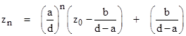
The preceding expressions for the nth iterate of a linear fractional transformation assume the LFT has two distinct fixed points. More generally, given any linear fractional recurrence relation

we can derive a closed-form expression for the nth iterate z_n in terms of n and z₀. These expressions are summarized in Table 1 for the various cases. Notice that cases 2 and 3 are really linear transformations, since c = 0. Case 4 corresponds to the case when the two fixed points of the LFT are co-incident. In this "parabolic" case, if a + d = 0 then the LFT reduces to Case 1 with ad–bc = 0. Case 5 is the general case with two distinct fixed points. In this case, if a + d = 0 then σ = 0 and K = –1.

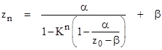
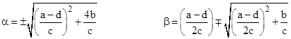
It's also interesting to note that the general expression for Case 5 can be written in the form

so if we define the LFT

we have

Setting n = 1 and noting that f(z₀) = z₁, we have

which shows that f(z) is conjugate to the simple function Kz. It's interesting to note that α + β is the "conjugate" of β, and so h(z) can be expressed as

where

Therefore, if c = 0, then either h(z) = 0 or h(z) is undefined.

3 General Periodicity Condition

It can be shown (see article on rational sines) that the sequence of iterates z_k of an LFT is cyclical with a period of m (meaning that z_k+m = z_k for every integer n) if and only if

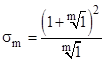
for some integer k. The "periodic" values of σ can also be expressed algebraically in the form

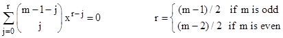
It's interesting that each –σ_m is a root of the polynomial

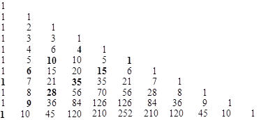
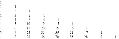
This gives the roots of polynomials whose coefficients are diagonal elements of Pascal's triangle

For example, the five roots of the quintic x⁵ + 9x⁴+ 28x³ + 35x² + 15x + 1 are given by

and the three roots of the cubic x³ + 6x² + 10 + 4 are given by

The factorizations of the first 24 "periodic σ polynomials" are presented in Table 2. If F_k(x) denotes the polynomial with roots –σ_k, then F_m(x) divides F_n(x) if and only if m divides n. This follows from the fact that if an LFT is cyclical with a period of m, and if m divides n, then the LFT also is has a (not fundamental) period of n.

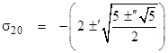
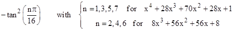
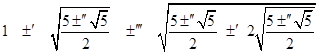
Although the roots of each F_m(x) are easily expressed in trigonometric form, it's interesting to note the following algebraic solutions for m = 16, 20, and 24. These are found by solving the quartic factor of F_m(x) in each case, which gives the four values of σ corresponding to the LFTs with a fundamental period of p in each case.

Since the condition for having period m is entirely a function of σ, and two LFTs are similar if they have the same σ, if follows that the number of dissimilar LFT groups of order m is equal to the number of distinct values 4cos²(kπ/m). This is clearly half the number of integers less than and co-prime to m, so the number is f(m)/2, half the Euler totient function.

If an LFT has a periodic of m, then it is said to generate a (cyclic) group order m.

4 The σ Form

Given any linear fractional transformation f(z) = (az+b)/(cz+d) with ad ¹ bc and (a+d),c ¹ 0, we can solve the similarity parameter equation

for b to give

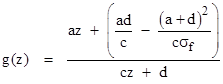
It follows that the function

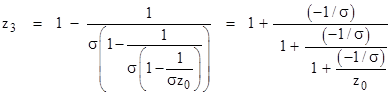
is similar to f(z) for any choice of parameters a, b, and c (provided c and a+d do not equal zero). In particular, setting d=0 and a=c gives the simple form

This implies that the iterates of g(z) are given as simple continued fractions. For example, z₃ can be expressed as a function of z₀ as follows

5 Self-Similar Iterations

Given any linear fractional transformation f(z) = (az+b)/(cz+d), the first iterate of this function is

which has the similarity parameter

Therefore, the sequence of similarity parameters of the iterates of a linear fractional transformation satisfy the non-linear recurrence

Setting σ_k+1 = σ_k and solving the resulting quadratic shows that all the iterates of f are similar to each other if and only if σ = 1 or 4. The recurrence gives a chaotic sequence for a range of initial values, similar to the logistic equation.

6 The λ Form

One of the most interesting special forms of linear fractional transformations is

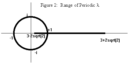
Every (non-degenerate) LFT is similar to an LFT of this special form. In fact, it is similar to exactly two LFTs of this form, because this special LFT is similar to the LFT given by replacing λ with 1/λ. This implies the important fact that every periodic λ is either purely real or it is complex with a magnitude of 1 (i.e., on the unit circle). Figure 2 shows the range of periodic l values in the complex plane.

mob3

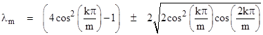
The periodicity condition for this form is that z_n+m = z_n if and only if λ has one of the values

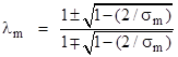
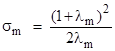
where k is an integer. These values can also be expressed in terms of the corresponding similarity parameters as

which implies

We saw in the previous section that iterations of f have the same similarity parameter σ if and only if σ equals 1 or 4. These values of σ gives the following values for the corresponding λ forms

Note that these are the extreme values of periodic λ on the imaginary axis and the real axis, respectively (excluding –1).

The values of λ that give periodic LFT iterations are the roots of a special set of polynomials whose coefficients are members of a generalized set of binomial coefficients. Each member of the generalized family of coefficient sets is denoted by a three-index symbol, defined as follows

Based on this definition, the following properties can be established:

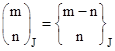
Symmetry:

Unit Plane:

Binomial Plane:

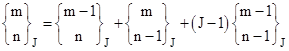
Recurrence Relation:

Column Relations:

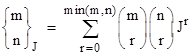
It is often more convenient to index the generalized coefficients in a manner similar to the indexing of the binomial coefficients. We define the generalized form as

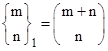
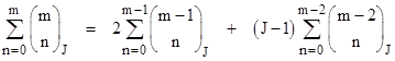
with the understanding that if no J subscript is specified, the value J=1 is implied (giving the normal binomial coefficients). In these terms we can establish the following recurrence relating the sums of successive rows of the coefficients:

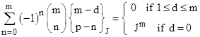
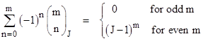
For J=1 this obviously gives the sums of the rows of binomial coefficients as powers of 2. The sum of the general row with alternating signs is given by

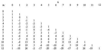
(with the stipulation that the sum equals 1 for the case J=1, m=0). The generalized coefficients with J = –1 are as follows

mob

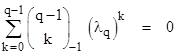
The roots of the polynomials with coefficients from a row of this table are precisely the values of λ for which the LFT is periodic. Specifically, letting λ_q denote the values of λ for which λ(1+z)/(1–z) has period q, we have

Since the coefficients are symmetrical, we know that if λ is a root, then so is 1/λ. The general form of the roots of these polynomials was given earlier in terms of the cosine function. However, several of these can be expressed purely algebraically. A list of these is presented in Table 3.

7 The Sum and Difference Form

Another interesting special form is

which has the convenient closed form expression

The periodicity condition for this form is

8 The Complement Form

Another interesting form of linear fractional transformation is

The values of a for which z_n+m = z_n are 4sin²(kπ/2m), k = 1, 2,...

9 The Diagonal Form

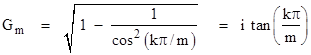
Another interesting form is

This LFT is similar to any other LFT with a σ such that

The values of G for which the LFT has a finite period m are

The values of –G_m² are precisely the roots of the polynomial whose coefficients are every second value in the mth row of Pascal's triangle. For example, consider the polynomial with coefficients taken from the 7th row

The three roots of the cubic x³ + 21x² + 35x +7 are –tan²(kπ/7) with k=1,2,3. If, on the other hand, we took every other coefficient from the 7th row beginning with the second column, we know that the three roots of the cubic 7x³ + 35x² + 21x + 1 are simply the inverses of the roots of the former polynomial, i.e., –1/tan²(kπ/7) with k = 1, 2, 3.

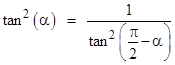
A convenient way of expressing these roots is to make use of the trigonometric identity

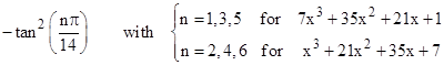
On this basis, we can say that the roots of the two polynomials with coefficients from the 7th row of Pascal's triangle are given by

Notice that we now have 2m instead of m in the denominator of the tangent. This same formulation works for even numbered rows as well. For example, the roots of the two polynomials taken from the 8th row are

10 Density of Real Iterates

Given the linear fractional recurrence

we can derive a closed-form expression for x_n that is particularly useful when the sequence is purely real. Beginning with the closed-form solution presented in Table 1 for the general case 5, we can substitute the trigonometric for the exponential form and arrive at the expression

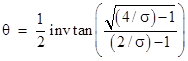
where we have defined the parameters

and

If we set x₀ = μ, then the expression for x_n reduces to

The function tan(x) is periodic modulo π, and assuming θ/π is irrational we can surmise that the values of nθ (mod π) for n = 0,1,2,...k... will approach an even distribution on the interval [0 , π] for sufficiently large k. Therefore, the asymptotic density of the iterates at any value x is proportional to the slope, i.e., derivative, of n with respect to x, since that is proportional to the number of n's that fall within a given interval Δx. The preceding equation gives

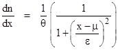
so the derivative of n with respect to x is

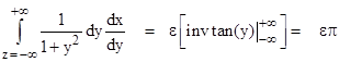
The asymptotic density of the iterates is proportional to this derivative, so we need only determine the appropriate scale factor to give the absolute density. The scale factor must be such that the integral of the density from x = –∞ to +∞ equals 1. In terms of the variable y = (x–μ)/ε, we know that

and since invtan(±∞) = ±π/2, it follows that

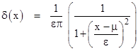
Therefore, the scale factor on 1/(1 + y²) must be 1/(επ), so the asymptotic density of iterates is given by

This is called the Cauchy distribution in probability theory. It's easy to show that half of the iterates will fall within the range μ ± ε, and two thirds of the iterates will fall within the range .

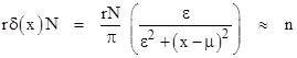
The Cauchy distribution has no well-defined mean or standard deviation, but the appearance of π in this density suggests that we could infer the value of π from a sequence of iterates. For example, if we compute N consecutive real-valued iterates of the linear fractional transformation f(x) = (ax+b)/(cx+d), and let n denote the number of these iterates that fall in the range –r/2 to +r/2 for some small real number r, then, provided f is not periodic, we expect the relation

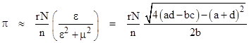
Re-arranging and inserting the expressions for ε and μ in terms of the linear fractional transformation coefficients a,b,c,d, this gives

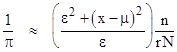
If we choose the coefficients such that (a–d)² = –4b(b+c), the right-hand factor equals unity and the equation reduces to π ≈ rN/n. A slightly different approach can be based on the density in the small range of width r around an arbitrary value of x

Thus we have

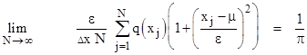
Now, this applies for any arbitrarily small range r centered on any value x, and in each case n represents the number of iterates that fall within that range. Hence if we consider k consecutive such ranges, and we add together the estimates of 1/π from each range, and divide by k, we get the average of 1/π for all of those ranges. This gives kr in the denominator, which is simply the entire range Δr of the k consecutive intervals. Consequently, for any finite range Δr and initial value x₀ we can compute 1/π from a series of iterates x₁, x₂, x₃, …, x_N by the formula

where Δx = x_max – x_min and q(x) = 1 or 0 accordingly as x is or is not in the range from x_min to x_max. This formula shows that we are essentially just computing the variance of the iterates, which behave (overall) like random samples from a Cauchy distribution, which is the normalized standard Cauchy distribution if μ = 0 and ε = 1. This occurs if and only if a = d and b = –c for non-zero values of a and b. Of course, the complete normalized standard Cauchy distribution

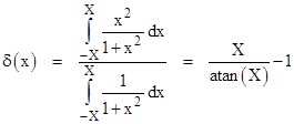
has no finite mean, standard deviation, or variance, but the truncated distribution over any finite range (–X,X) has the variance

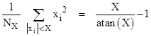
Hence for any linear fractional transformation of the form f(x) = (ax + b)/(–bx + a) for any non-zero real coefficients a,b, (provided f is not periodic, i.e., provided the inverse tangent of b/a is not a rational multiple of π) we can say that the variance of the iterates that fall within the range (–X,X) is

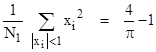
where N_X is the number of iterates in the summation. In particular, if we set X = 1, we have

The fact that the variance of the linear fractional iterates falling in the range from –1 to +1 does indeed converge on 4/π – 1 demonstrates that the values of nθ modulo π are (in the agregate) uniformly distributed over the interval 0 to π for most values of θ.

Table 1: Closed Form Expressions For nth Iterates of (az+b)/(cz+d)

Case 1: ad = bc, c ¹ 0