Harmonia Mensurarum

The second edition of Isaac Newton's Principia was published by Richard Bentley, the famous classical scholar and Master of Trinity College. Bentley was not universally well-liked (to put it mildly), and was certainly no scientist or mathematician, so it may seem odd that Newton chose him as his publisher, especially considering how many better-qualified men (such as David Gregory) would have jumped at the chance. True, Bentley had delivered a series of lectures in 1692 using Newton's theories to "prove" the existence of an intelligent creator - exactly the kind of thinking that appealed to Newton - but it was still an odd partnership. When he was later asked why he had chosen Bentley as publisher, Newton answered (probably in jest) that Bentley "was covetous & loved money & therefore I lett him that he might get money". That may be, but it's also possible that Newton (then 67) was not eager to engage a publisher who would subject the book to detailed scrutiny. He seems to have hoped to correct a few typos and ship it off to the printers, and with Bentley as editor this is probably what would have happened.

Whatever Newton's intentions may have been, events took a different turn when Bentley enlisted the bright young (27) mathematician Roger Cotes (1682-1716) to do the actual editing of Newton's great work. Cotes was the newly appointed professor of astronomy at Trinity College, a position he had gained with Bentley's support. It soon became clear to Newton that this new edition was not going to be an easy ride. Shortly after the project began, Cotes wrote to inform Newton of two errors he had found in a table of integrals referenced in the corollary of Proposition XCI. In reply, Newton tried to dampen his enthusiasm

I thank you for your letter and the corrections... I would not have you be at the trouble of examining all the demonstrations in the Principia. It's impossible to print the book without some faults, and if you print by the copy sent you, correcting only such faults as occur in reading over the sheets to correct them as they are printed off, you will have labor more than it's fit to give you.

Apparently a cursory approach to the new edition wasn't what Cotes had expected. He showed the letter to Bentley, and asked him to clarify the scope of the task. Bentley wrote back to Newton:

You need not be so shy of giving Mr. Cotes too much trouble. He has more esteem for you and more obligations to you than to think that trouble too grievous. But however he does it at my orders, to whom he owes more than that. And so pray you, be easy as to that. We will take care that no little slip in a calculation shall pass this fine edition.

This zeal may have been a bit threatening, from Newton's point of view, but eventually he warmed to the task, and Cotes succeeded in getting Newton to thoroughly re-work much of Books II and III, including the section on the resistance of fluids to motion and the extremely difficult sections on the lunar motion (which Newton said made his head ache). Newton also added the famous General Scholium to the end of Book III. Work on the Principia occupied Cotes for nearly four years. Interestingly, the notions of "action at a distance" and gravity as an innate property of matter, commonly attributed to Newton, were actually first clearly articulated by Cotes in his preface to the second edition.

Cotes died at the age of 34, prompting Newton to make the famous remark that "if he had lived, we might have known something". Although Cotes published almost no original work during his life, some of his writings were published posthumously by his uncle. Among the results that tend to support Newton's comment, we find that Cotes in 1714 was the first to note the fundamental identity

where i = √–1. A generation later the great Swiss mathematician Euler deduced the same result and expressed it in the more familiar form

This identity can be seen as an expression of the correspondence between circular and hyperbolic measures, between exponential and trigonometric measures, and between orthogonal and polar measures, not to mention between real and complex measures, all of which seemed to be within Cotes' grasp. He named the treatise containing this result Harmonia Mensurarum, meaning "harmony of measures".

Another interesting and "harmonious" result found by Cotes concerns the points of intersection between a pencil of straight lines and an algebraic curve. Recall that an algebraic curve is defined by a function f(x,y) = 0 where f is a polynomial in the variables x and y. This means that f(x,y) is the sum of terms of the form c_m,n x^myⁿ. The largest value of m+n for any term with non-zero coefficient is called the degree of f. An algebraic curve of the first degree is a straight line, whereas the algebraic curves of degree 2 are the conics, i.e., circles, ellipses, hyperbolas, parabolas. We can have algebraic curves of any degree, including cubics, quartics, etc.

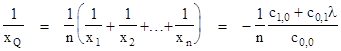
Given an arbitrary algebraic curve of degree n, and an arbitrary point O on the plane, suppose a straight line through the point O intersects the curve at n points, labeled P₁, P₂, ... P_d , and let r_j denote the distance from O to the point P_j. Now mark the point Q on the line at the distance r_q from O, where r_q is the harmonic mean of r₁, r₂, ..., r_n. If we repeat this process for many different lines through O (each intersecting the curve at n points), Cotes stated that the constructed "Q" points will all lie on a straight line.

Oddly enough, since this theorem involves the harmonic mean, the historian of mathematics W.W. Rouse Ball evidently concluded that this was the theorem from which Cotes' Harmonia Mensurarum took its name, and this claim is repeated in Boyer's history. However, Hollingdale notes that this result actually was part of a different treatise, called On the Nature of Curves.

In any case, it's a nice result, and at first glance seems as if it might be quite difficult to prove - even assuming it's true, which may not be intuitively obvious. We can easily imagine plane curves for which the theorem does not hold, but they are not algebraic curves. (It turns out that, in effect, we could almost use Cotes' theorem to define algebraic curves.) Another potential objection is that some of the lines through the point O may intersect an algebraic curve of degree d in d points, whereas other lines through O may not, so it may seem that the theorem must break down at some point.

However, this theorem is actually quite easy to prove, provided we accept the fundamental theorem of algebra, which assures us that a line always intersects an algebraic curve of degree n in exactly n points (not necessarily distinct), with the understanding that the points of intersection may have complex coefficients. To prove the theorem, we can, without loss of generality, set the point O at the origin of x,y coordinates, in terms of which our algebraic curve is defined by a polynomial of the form

Also, a straight line through the point O has the equation y = λx for some constant λ. To find the points of intersection we substitute for y in the above polynomial to arrive at the single-variable polynomial of degree n

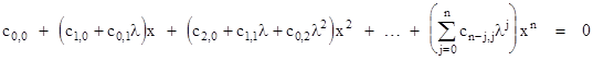
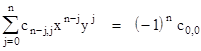
Since this polynomial is of degree n, it has n (possibly complex) roots, and these correspond to the x coordinates of the n points of intersection. Now, recall from the basic theory of equations that for the general polynomial of degree n

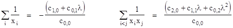
the value of C_j/C_n equals the sum of all products of the roots taken j at a time. For example, C_n-1/C_n is just the sum of the roots, whereas C₀/C_n is just the product of the roots. Likewise, C₁/C_n is the sum of all products of n–1 roots. It follows that C₁/C₀ is the (negative) sum of the reciprocals of the roots.

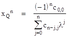
The distances from O of points on the line are all directly proportional to the x coordinates of those points, so we can simply work with the x coordinates of the intersections points and compute the harmonic mean to give the x coordinate of the "Q" point. Thus we have

The point Q is also on the line y = λx, so we have y_Q = λx_Q.  Substituting y_Q/x_Q for λ in the above expression and re-arranging gives

Since n and the coefficients c_i,j are constants for a given algebraic curve, we see that the coordinates of the Q points all satisfy this same equation of a line, regardless of the value of k, so this proves Cotes' theorem. Notice that this works for all lines through the point O, even those that don't have a real point of intersection with the curve, because we are allowing the coordinates of the intersection points to be complex.

As a simple illustration, consider the algebraic curve of degree 2 defined by the polynomial

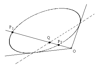
This gives an ellipse as shown in the figure below.

For any line through the point O that intersects the ellipse at the points P₁ and P₂ we can find the point Q such that

The dashed line in the figure represents the locus of such points Q for all possible straight lines through the point O. This locus extends outside the ellipse, into the region where there are no real intersections between the ellipse and a line through O, but in this region there are complex points of intersection, and the distance OQ computed from harmonic mean of those distances is purely real-valued, and places the point Q on the dashed line.

Incidentally, the writings of Cotes on the subject of Newton's fluents and fluxions, as well as the measures of curves and integration formulae (see The Prismoidal Formula), were evidently known to Edgar Allan Poe, who included among his marginal notes (Marginalia - Part I, 1844) the whimsical comment

I think I will set about a lyric on the Quadrature of Curves--or the Arithmetic of Infinites. Cotes, however, supplies me a ready-made title, in his "Harmonia Mensurarum," and there is no reason why I should not be fluent, at least, upon the fluents of fractional expressions.

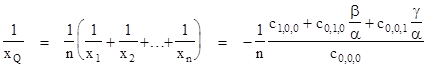
The theorem can immediately be generalized to higher dimensions. For example, given any algebraic surface defined by the polynomial function f(x,y,z) = 0 of degree n, we can construct a straight line from the origin O intersecting the surface at n points. If we denote by Q the point on this line whose distance from the origin is the harmonic mean of the distances to the n points of intersection with the surface, the theorem asserts that the locus of such Q points is a flat plane. This can be demonstrated by essentially the same presented above. The equation of the line can be expressed in parametric form by the equations

for constants α, β, γ, so we have y = (β/α)x, z = (γ/α)x. Substituting these expressions for x and y into the polynomial f(x,y,z) = 0 gives a polynomial in x of degree n, and the lowest order terms are

By the same reasoning as before, we have

Multiplying through by X_Q gives the result

which is the equation of a plane, independent of the coefficients α, β, γ of the line. Hence the locus of "Q" points is a plane.

In general, the locus of points whose distance along a line from a fixed point O in d-dimensional space is the harmonic mean of the distances along the line from the point O to all the points of intersection of the line with a fixed algebraic surface in the d coordinates is a flat d–1 dimensional space.

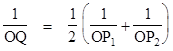
This theorem can also be extended in other ways. For example, given an algebraic plane curve of degree n, consider a pencil of lines through an arbitrary point O. Each line intersects with the curve in n points (possibly with complex coordinates). For any given line through the point O, let r₁, r₂, ..., r_n denote the distances from O to the points of intersection with the curve, and define the point Q on this line at a distance r_Q from the point O by the equation

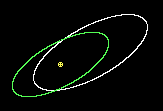
In other words, 1/r_Q² is the average of all products of two distinct inverses of the distances from O to the curve. In this case it's easy to show that the locus of the "Q" points for all the lines through O is a central conic around O. Of course, if the original given curve itself is of degree n = 2 (meaning that it is a conic), then each line through O intersections with the curve at just two points, at the distances r₁ and r₂, and in this case r_Q is just the algebraic mean of those two distances.  The figure below shows an ellipse in white and the locus of points in green such that the distance from the origin along any line through the origin is the geometric mean of the two distances to the ellipse along that line.

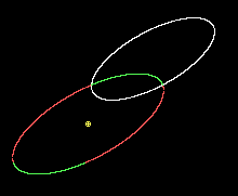
If the origin point is outside the given (white) ellipse, the result is still applicable, but in such a case the coordinates of the intersection points between the ray from the origin and the white ellipse are complex for rays outside the tangent rays. Nevertheless, there are still two intersection points, and the geometric mean of the distances is real, following the same ellipse as shown in red below.

For n > 2 the above formulas give r_Q as the average of the inverses of all products of two distances to the given curve, but we can also easily derive the formulas for r_Q defined as the geometric mean of all the distances r₁, r₂,.., r_n from the point O to the curve for all values of n. (This is equivalent to the previous case when n = 2, but not for n > 2.) For the general plane polynomial f(x,y) of degree n we can set y = λx to give the polynomial of x values of the points of intersection between the curve and a line through the origin with slope λ. The result is

To set r_Q equal to the geometric means of the n distances, we must set x_Q to the geometric mean of the roots of this equation, so we have

where λ = y_Q/x_Q. Multiplying through by the denominator on the right side, we have the locus of "Q" points:

Consequently the locus is a central homogeneous curve of degree n. Moreover, it is identical to the original plane curve, except that all the terms of degree 1 through n–1 are deleted.

As a simple illustration, suppose the given plane curve is the hyperbola

Expanding this into polynomial form gives

Every line through the origin intersects this curve in two points (possibly with complex coordinates), and if we mark on each line the points at a distance from the origin equal to the geometric mean of the distances of the two points of intersection with the hyperbola, then the locus of all these points is the hyperbola given by the above polynomial with the terms of the first degree deleted, i.e., the reduced polynomial

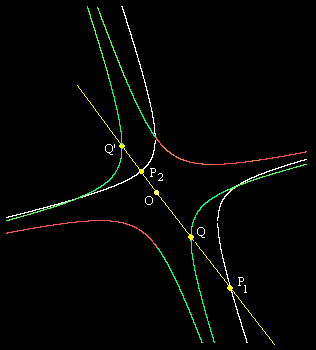
A plot of these curves is shown below.

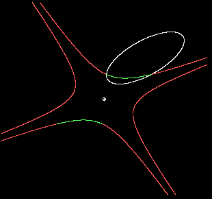
The white hyperbola is the original plane curve, and the point marked "O" is the origin. A sample line drawn through the origin is shown in yellow, intersecting the white hyperbola at the points P₁ and P₂. We then mark the points Q and Q' on this line at a distance given by the geometric mean of the distances from the origin to the points P₁ and P₂. As we rotate the line through O, these Q and Q' values generate the hyperbola shown in green and red. The red portions are where the intersection points have complex coordinates. Notice that we generate two conjugate hyperbolas by setting the reduced polynomial to +121/25 or –121/25.

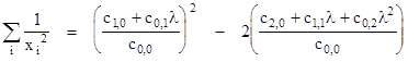
In this same way we can characterize the locus of points generated by any symmetrical function of the distances from a point to a given curve.  As an example, suppose we define 1/r_Qⁿ as the means of the inverse squares of the distances along a line from the origin to the n points of intersection with the given curve. Since we have

it follows that

Equating this to n/x_Qⁿ and clearing fractions (with λ = y_Q/x_Q) gives the conic locus

In this case the Q locus need not have the same discriminant as the original curve. As an example, the figure below shows the locus of points (green) whose inverse-square distances are the mean of the inverse squares of the distances to the curve (white).

The red lines are generated by the same condition, applied to the complex points of intersection.

Return to MathPages Main Menu