Integrating The Bell Curve

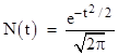
The standard normal distribution (first investigated in relation to probability theory by Abraham de Moivre around 1721) is

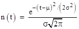
More generally, replacing t with (t-μ) and re-scaling with an arbitrary factor of σ, the normal density function with mean of μ and standard deviation of σ is

This standard normal distribution N(t) – sometimes called the “bell curve” because of its shape – arises in many important applications. For example, the probability that a sample drawn from a normally distributed population will fall within a given range of t equals the area under the curve for that range. Hence we often need to integrate the bell curve to find probabilities. Aside from re-scaling, the basic function to be integrated is exp(–t²). Determining the closed-form expression for the integral of exp(–t²) from t = –∞ to +∞ is fairly easy, but it's more difficult to evaluate the area under a limited portion of the curve, such as the small tail of the distribution for t greater than some large value. In fact, there is no exact "closed form" expression for the value of this integral over an arbitrary range. There are, however, various effective techniques for evaluating this integral, some of which illustrate the usefulness of divergent series (also known as asymptotic series).

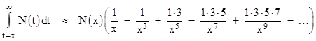
Expanding the function exp(–t²) into a series and integrating term by term is one simple way of deriving an expression for the integral over a specific range. This gives

Interestingly, this shows that the integral is basically the scalar product of two infinite-dimensional vectors, one having the components (1, –1/3, 1/5, –1/7, …) and the other having the components (1, u²/1!, u⁴/2!, u⁶/3!, …). The first ten terms of this series give the area under the curve from t = –1 to 1 with a precision of ten significant digits, but to achieve the same precision up to t = 3 requires 25 terms. Moreover, we are often interested in the area under the “tail” of the curve, i.e., the area in the range t = x to ∞, which is (half of) the complement of the above integral. As a result, we lose precision for large values of x. Therefore, this approach isn’t very suitable for determining areas under the normal curve far from the mean.

An alternative approach (leading to the concept of asymptotic series) is to make use of the fact that, although N(t) cannot be integrated in closed form, there are functions that asymptotically approach N(t) in certain ranges and that do have closed form integrals. For example, consider the two functions

As t becomes large, these functions obviously converge on N(t), with L(t) approaching from below and U(t) from above. These functions have nice closed-form integrals, so they can be used to provide bounds on the integral of N(t). Let A(x) denote the integral of N(t), i.e., the area under the "tail" of the Normal curve from t = x to t = +∞. The integrals of L and U gives the following lower and upper bounds, respectively:

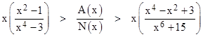
We can refine these further by noting that a characteristic of N(t) is that almost all the area from x to +∞ is very close to x. Therefore, if we multiply the lower bound by the ratio N(x)/L(x) and the upper bound by the ratio N(x)/U(x), we will just slightly overcompensate in both cases. This gives the improved bounds

For example, the bounds on the "six-sigma" tail area given by these two equations are (9.8680)10^–10 > A(6) > (9.8654)^–10.

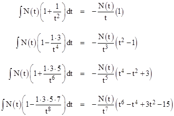
Returning to the upper and lower approximation functions given by (2), notice that they are just special cases of a family of exact integrals of functions that asymptotically approach N(x). We have the following indefinite integrals

Evaluating these from t = x to +∞ gives an alternating sequence of upper and lower bounds on the integrals of N(t) for t > x. Note that the denominator on the left hand side in each successive formula increases by a factor of t², but the numerator increases factorially. As a result, it's clear that for any fixed value of t there is a limit to how much precision we can achieve by going to higher orders.

For example, if we want to evaluate the tail of the normal distribution above 3 (standard deviations), each successive denominator increases by at least 9, so the optimum approximation we can achieve (in this direct way) would be the next one after those shown above, for which the numerator would be 1∙3∙5∙7∙9. Subsequent approximations would have the numerator multiplied by 11, 13, and so on, whereas the denominator would still just be increased by a factor of 9 on each step, so the error would get bigger rather than smaller. This is a characteristic of asymptotic series: for a given argument the error becomes smaller as terms are added, until reaching a minimum, beyond which the error becomes larger. Thus, the series representation

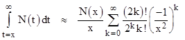
is actually divergent for all x, but the error is smaller than the first neglected term (recalling that consecutive partial sums give strict upper and lower bounds), so by selecting the appropriate number of terms for a given x we can often achieve good results. To quantify the best precision that we can achieve by the simple application of this series (without interpolation), note that the denominator increases by a factor of x² in each term, so the tightest bounds are between the two terms for which the numerator increases by a factor of (approximately) x². The tolerance is then equal to the difference between those two terms. The asymptotic series can be written as

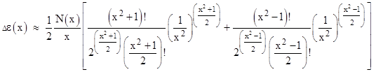
Hence for any given value of x the two smallest terms will be those with k–1 and k such that 2k – 1 = x². We initially think of integer x values, so the factorials are defined, but later we will revert to gamma functions so the expressions apply to any x. Inserting this value for k into the two consecutive terms gives the difference

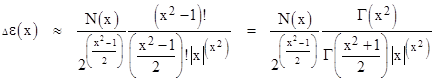
The two consecutive terms have opposite signs, so we add their magnitudes to get the difference. Also, the two terms are equal, so half the sum reduces to

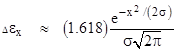
(It’s interesting that there exist two consecutive terms with exactly equal magnitude if and only if x² equals 2k – 1 for some integer k, so there is a “quantum condition” on x.) The natural log of this error is virtually a straight line when plotted against x², so we find that the error is proportional to a normal distribution, i.e.,

where σ equals approximately ln(2). From this we see that the divergent series can give the integral of the normal curve from x to infinity only to an accuracy of about 0.5% for values of x near three standard deviations above the mean, but it can give the integral for x near six standard deviations accurate to nine significant digits.

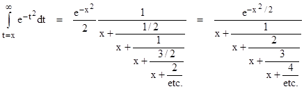
Yet another approach to evaluating the area under the bell curve, and one that is convergent (in a sense) for all x, is to use the continued fraction originally found by Laplace:

However, to say that these expressions are “convergent” is slightly misleading, as is the form of the equations themselves, because it suggests that we can sequentially compute more and more accurate results by just adding more individual terms, which is not really the case. To evaluate a continued fraction we must choose some low point on the fraction and work upwards. For example, to evaluate the above fraction for a given value of x, we might decide to begin at the third level, and proceed upwards by the following sequence of operations: take the reciprocal of x, multiply by 3, add x, take the reciprocal, multiply by 2, add x, take the reciprocal, multiply by 1, add x, take the reciprocal, and then finally multiply by exp(–x²/2). This gives the third-level approximation, but if we want the fourth-level approximation there is no simple way of building on the third-level result. We must begin all over again, starting with x, climb back through all the levels. The expression is “convergent” only in the sense that it represents a sequence of distinct calculations, and the error approaches zero as we proceed from one calculation to the next, but the error does not approach zero for any individual calculation. If an ordinary summation represents a “series”, a continued fraction expression actually represents a meta-series of series.

Incidentally, the "bell curve" has sometimes become the subject of spirited public debate because of the uses to which it has been put. As with any mathematical model, its applicability to any particular situation is subject to question, and it can certainly be used inappropriately. The fields of probability and statistics have always struggled to establish principles that would justify their applicability (or lack thereof) in various circumstances. It sometimes surprises people who routinely rely on statistical methods and probabilistic analyses that there is no general agreement among mathematicians as to what (if anything) probability actually means in a utilitarian sense. On one level, probabilistic formulas such as the normal distribution can be used for purely descriptive purposes, e.g., to summarize the observed variation in resilience of a billion paper clips. However, even for such purely descriptive purposes, the use of the “bell curve” has been seen as odious, particularly when applied to the description of human beings. It is, in some way, de-humanizing to quantify and parameterize people – their attributes and capacities. This sort of mathematization has caused the term “bell curve” to have distinctly pernicious connotations for many people.

A more technical kind of objection to the “bell curve” arises when we pass from purely descriptive uses to predictive applications. For example, after describing in terms of a normal distribution the resiliency observed in one billion paper clips, we may be tempted to use the formula to assess the likely resilience of the next paper clips we encounter. A careful statistician will point out that our formula is applicable only provided the next paper clips are from the same population as the original set, but of course this is tautological, because "being from the same population" is defined as meaning that the same distribution formula applies. When we pass from the descriptive to the predictive application of statistical formulas we inevitably face this difficulty. The statistician can only assert the tautology that future events will conform to a given mathematical model if they conform to that mathematical model. This is reminiscent of the summary of Newton's laws motion: Objects move at constant speed in a straight line except when they don't.

Many people have decried the indiscriminate application of "the bell curve" (and other similar models) for predictive purposes, in the spirit of the fiduciary reminder that past history is no guarantee of future performance. No matter how much uniformity and consistency we have observed in the past, it is always possible that our next observation will be completely "out of population". (Of course, by the nature of probabilistic models, no sequence of observations can be entirely ruled out, even if we are dealing with a single population with a given distribution.) Nevertheless, we do develop expectations based on our experience, and this is at least successful enough in general for us to continue doing it. Also there seems to be no alternative. We have no right to expect, a priori, that our experience will exhibit any kind of coherence or comprehensibility, but we do seem to find patterns that persist at least to some extent. Some authors on this subject seem to suggest that we would be better served by not using models of past experience to make predictions... but their alternatives (when they offer any) invariably amount to simply advocating different models (or meta-models) of past experience, which of course are not exempt from the same criticisms. Still, the exhortation to consider possible meta-models (and meta-meta models) is well taken. In other words, rather than just focusing on one population and its distribution, it may be useful to consider the population of populations and its distribution. This is especially important at the "tails" of the distribution, when the probability of encountering a member of a completely different population may greatly outweigh the probability of encountering an out-lier from the original population. (One is reminded of the statistician who announced after much calculation that he was 90% certain that the probability of system failure was less than 10^–9.)

It's interesting how, in a sense, the divergent series representations of the normal distribution serve as mathematical models of both the viability and the limitations of formally derived expectations. The series expressions arise from purely formal considerations, and they do indeed converge on the underlying structure - but only to a limited extent, beyond which they diverge into meaninglessness.

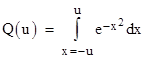
One might wonder if it’s possible to adapt the usual method for evaluating the basic integral

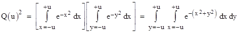
for u = ∞ and use this method to compute the integral for finite ranges. Recall that the usual method is to consider the square of the integral as the product of two independent integrals

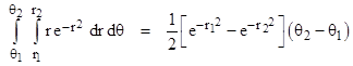
Converting to polar coordinates with x = r cos(θ) and y = r sin(θ), and noting that the area differential is dA = dx dy = r dθ dr, this double integral can be written as

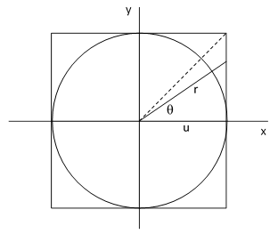
for any fixed ranges of θ and r. However, the region of integration of the previous double integral in terms of xy coordinates is square, whereas the region of integration of this double integral in terms of polar coordinates is circular (or a slice of a circle). In the special case of u = ∞ the region of integration is the entire xy plane, and we can achieve the same coverage with polar coordinates by taking θ₁ = r₁ = 0 and θ₂ = 2π, and r₂ = ∞. Inserting these values into the polar double integral gives the result π, and hence we have the well-known result that the single integral is the square root of π. But if a is finite, the task of integrating over the square region in terms of polar coordinates is more difficult, because the radial range becomes a function of the angle, as can be seen from the figure below.

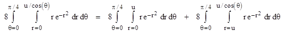
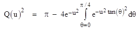
By symmetry we need evaluate only the integral over the half-quadrant from θ = 0 to π/4, in which the radial range is related to the angle by r = u/cos(θ), and then multiply the result by 8 to cover the entire square. Thus we must evaluate the integral

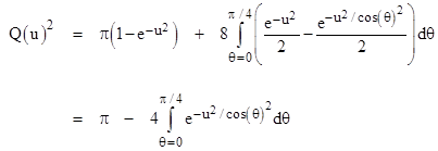
Evaluating the first double integral on the right side, and the interior integral of the second, we have

Making use of the identity cos(θ)² = 1/(1+tan(θ)²), this can be written as

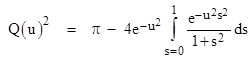
In terms of the variable s = tan(θ) this becomes

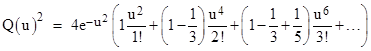
Expanding the integrand into a series and evaluating the integral term by term, we get

This doesn’t lead to a very efficient formula, but it’s interesting that the integral can be written in the form

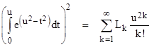
Thus we have the exponential generating function for the partial sums of the Leibniz series

where

By comparison, equation (1) shows that the un-squared integral (and without the factor of exp(u²)) is the generating function of the individual terms of the Leibniz series.

Return to MathPages Main Menu