Force Laws and Maxwell's Equations

While speaking of this state, I must immediately call your attention to the curious fact that, although we never lose sight of it, we need by no means go far in attempting to form an image of it and, in fact, we cannot say much about it.

                                                              Hendrik Lorentz, 1909

Perhaps the most rudimentary scientific observation is that material objects exhibit a natural tendency to move in certain circumstances. For example, objects near the surface of the Earth tend to move in the local "downward" direction, i.e., toward the Earth's center. The Newtonian approach to describing such tendencies was to imagine a "force field" representing a vectorial force per unit charge that is applied to any particle at any given point, and then to postulate that the acceleration vector of each particle equals the applied force divided by the particle's inertial mass. Thus the "charge" of a particle determines how strongly that particle couples with a particular kind of force field, whereas the inertial mass determines how susceptible the particle's velocity is to arbitrary applied forces. In the case of gravity, the coupling charge happens to be the same as the inertial mass, denoted by m, but for electric and magnetic forces the coupling charge q differs from m.

Since the coupling charge and the response coefficient for gravity are identical, it follows that gravity can only operate in a single directional sense, because changing the sign of m for a particle would reverse the sense of both the coupling and the response, leaving the particle's overall behavior unchanged. In other words, if we considered gravitation to apply a repulsive force to a certain particle by setting the particle's coupling charge to –m, we would also set its inertial coefficient to -m, so the particle would still accelerate into the applied force. Of course, the identity of the gravitational coupling and response coefficients not only implies a unique directional sense, it implies a unique quantitative response for all material particles, regardless of m. In contrast, the electric and magnetic coupling charge q is separately specifiable from the inertial coefficient m, so by changing the sign of q while leaving m constant we can represent either negative or positive response, and by changing the ratio of q/m we can scale the quantitative response.

According to this classical picture, a small test particle with mass m and electric charge q at a given location in space is subject to a vectorial force f given by

where g is the gravitational field vector, E is the electric field vector, and B is the magnetic field vector at the given location, and v is the velocity vector of the test particle. (See Appendix 1 for a review of vector products such as the cross product denoted by v x B.) Strictly speaking, the force on a discrete charged particle must also include a “radiation reaction” term to account for the effect of the particle’s own field on its state of motion, but this force is significant only for large accelerations, and is usually neglected in the classical Maxwell-Lorentz formulation of electrodynamics. We will return to this important subject in Section 9.10, but in the present section we focus on the classical formulation.

As noted above, the acceleration vector a of the particle is simply f/m, so we have the equation of motion

Given the mass, charge, and initial position and velocity of a test particle, and the vectors g,E,B for every point in the vicinity of the particle, this equation enables us to compute the particle's subsequent motion. Notice that acceleration of a test particle due to gravity is independent of the particle's properties and state of motion (to the first approximation), whereas the accelerations due to the electric and magnetic fields are both proportional to the particle's charge divided by it's inertial mass. In addition, the contribution of the magnetic field is a function of the particle's velocity. This dependence on the state of motion has important consequences, and leads naturally to the unification of the electric and magnetic fields, but before describing these effects it's worthwhile to briefly review the effect of the classical gravitational field on the motion of a particle.

The gravitational acceleration field g at a point p due to a distant particle of mass m was specified classically by Newton's law

where r is the displacement vector (of magnitude r) from the mass particle to the point p. Noting that r² = x² + y² + z² and r = ix + jy + kz, it's straightforward to verify that the divergence of the gravitational field g vanishes at any point p away from the mass, i.e., we have

(See Appendix 3 for a review of the “dell” differential operator notation.) The field due to multiple mass particles is just the sum of the individual fields, so the divergence of g due to any configuration of matter vanishes at every point in empty space. Now, the field is singular (infinite) at any point containing a finite amount of mass, so we can't express the field due to a mass point precisely at the point. However, if we postulate a continuous distribution of gravitational charge (i.e., mass), with a density ρ_g specified at every point in a region, then it can be shown that the gravitational acceleration field at every point satisfies the equation

Incidentally, if we define the gravitational potential (a scalar field) due to any particle of mass as φ = –m/r where r is the distance from the source particle (and noting that the potential due to multiple particles is simply additive), it's easy to show that

so equations (3) and (4) can be expressed equivalently in terms of the potential, in which case they are called Laplace's equation and Poisson's equation, respectively. The equation of motion for a test particle in the absence of any electromagnetic effects is simply a = g, so equation (2) gives the three components

To illustrate the use of these equations of motion, consider a circular path for our test particle, given by

In this case we see that r is constant and the second derivatives of x and y are –rω²sin(ωt) and –rω²cos(ωt) respectively. The equation of motion for z is identically satisfied and the equations for x and y both reduce to r³ω² = m, which is Kepler's third law for circular orbits.

Newton's analysis of gravity into a vectorial force field and an inertial response was spectacularly successful in quantifying the effects of gravity, and by the beginning of the 20th century this approach was able to account for nearly all astronomical phenomena in the solar system within the limits of observational accuracy (the only notable exception being a slightly anomalous precession in the orbit of the planet Mercury, as discussed in Section 6.2). Encouraged by this success, scientists attempted to represent the other forces of nature in a similar way.

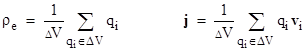
The next two most obvious forces that apply to material bodies are the electric and magnetic forces, represented by the last two terms in equation (1a). If we imagine that space is filled with a virtually continuous mist of infinitesimal electrical charges q_i with velocities v_i, then we can define the classical macroscopic charge density ρ_e and current density j within a given incremental volume ΔV as

For the remainder of this section we will omit the subscript "e" with the understanding the ρ signifies the electric charge density. Assuming all the infinitesimal charges within the incremental volume have essentially the same velocity with components dx/dt, etc., the individual components of the current density are

Maxwell's equations for the electro-magnetic fields are

where E is the electric field and B is the magnetic field. Equations (5a) and (5b) suggest that the electric and magnetic fields are similar to the gravitational field g, since the divergences at each point equal the respective charge densities, with the difference being that the electric charge density may be positive or negative, and there does not exist (as far as we know) an isolated magnetic charge, i.e., no magnetic monopoles. Equations (5a) and (5b) are both static equations, in the sense that they do not involve the time parameter. By themselves they could be taken to indicate that the electric and magnetic fields are each individually similar to Newton's conception of the gravitational field, i.e., instantaneous "force-at-a-distance". (On this static basis we would presumably never have identified the magnetic field at all, assuming magnetic monopoles don't exist, and that the universe is not subject to any boundary conditions that caused B to be non-zero.)

However, equations (5c) and (5d) reveal a completely different aspect of the E and B fields, namely, that they are dynamically linked together, so the fields are not only functions of each other, but their definitions explicitly involve changes in time. Recall that the Newtonian gravitational field g was defined totally by the instantaneous spatial condition expressed by

so at any given instant the Newtonian gravitational field is totally determined by the spatial distribution of mass in that instant, consistent with the notion that simultaneity is absolute. In contrast, Maxwell's equations indicate that the fields E and B depend not only on the distribution of charge at a given putative "instant", but also on the movement of charge (i.e., the current density) and on the rates of change of the fields themselves at that "instant".

Since these equations contain a mixture of partial derivatives of the fields E and B with respect to the temporal as well as the spatial coordinates, dimensional consistency requires that the effective units of space and time must have a fixed relation to each other, assuming the units of E and B have a fixed relation. Specifically, the ratio of space units to time units must equal the ratio of electrostatic and electromagnetic units (all with respect to any frame of reference in which the above equations are applicable). This is the reason we were able to write the above equations without constant coefficients, because the fixed absolute ratio between the effective units of measure of time and space enables us to specify all the variables x,y,z,t in the same units.

Furthermore, this fixed ratio of space to time units has an extremely important physical significance for electromagnetic fields in empty space, where ρ and j are both zero. To see this, take the curl of both sides of (5c), which gives

Now, for any arbitrary vector S it's easy to verify the identity

Therefore, we can apply this to the left hand side of the preceding equation, and noting that

in empty space, we are left with

Also, recall that the order of partial differentiation with respect to two parameters doesn't matter, so we can re-write the right-hand side of the above expression as

Finally, since (5d) gives

in empty space, the above equation becomes

Similarly we can show that

Equations (6a) and (6b) are just the classical wave equation, which implies that electromagnetic changes propagate through empty space at a speed of 1 when using consistent units of space and time. In terms of conventional units this must equal the ratio of the electrostatic and electromagnetic units, which gives the speed

where μ₀ and ε₀ are the permeability and permittivity of the vacuum. To some extent our choice of units is arbitrary, and in fact we conventionally define our units so that the permeability constant has the value

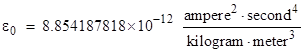
Since force has units of kg×m/sec² and charge has units of amp×sec, these conventions determine our units of force and charge, as well as distance, so we can then (theoretically) use Coulomb's law F = q₁q₂/(4π ε₀ r²) to determine the permittivity constant by measuring the static force that exists between known electric charges at a certain distance. The best experimental value is

Substituting these values into equation (7) gives

This constant of proportionality between the units of space and time is based entirely on electrostatic and electromagnetic measurements, and it follows from Maxwell's equations that electromagnetic waves propagate at the speed c in a vacuum. In Section 3.3 we review the history of attempts to measure the speed of light (which of course for most of human history was not known to be an electromagnetic phenomenon), but suffice it to say here that the best measured value for the speed of light is 299792457.4 m/sec, which agrees with the predicted propagation speed for electromagnetic waves based on the empirical value of permittivity and Maxwell's equations to nine significant digits.

This was Maxwell's greatest triumph, showing that electromagnetic waves propagate at the speed of light, from which we infer that light itself consists of electromagnetic waves, thereby unifying optics and electromagnetism. However, this magnificent result also presented physicists of the late 19th century with a puzzle that would baffle them for decades. Assuming the permittivity and permeability of the vacuum are the same when evaluated at rest with respect to any inertial frame of reference, and assuming Maxwell's equations are strictly valid in all inertial frames of reference, equation (7) implies that the speed of light must be independent of the frame of reference. This satisfies the Galilean principle of relativity, but is incompatible with the Galilean composition of velocities.

While attending "prep school" in Aarau, Switzerland in 1895, the young Einstein wondered “If one were to run after a ray of light as it travels, would its velocity thereby be decreased? If one were to run fast enough, would it no longer move at all?” Even the idea that light should go more quickly in one direction than in another seemed strange to him. The success of Maxwell’s equations only strengthened his belief that the speed of light is independent of the speed of the source (as in a wave theory), and yet he continued to have the impression that the speed must also be the same in all directions relative to the rest frame of the source (as in a ballistic theory), supported by the failure of the ether drift experiments. As Einstein later realized, these facts could be reconciled only if inertial coordinate systems are related by Lorentz transformations.

Writing out equations (5d) and (5a) explicitly, we have four partial differential equations

The above equations strongly suggest that the three components of the current density j and the charge density ρ ought to be combined into a single four-vector, such that each component is the incremental charge per volume multiplied by the respective component of the four-velocity of the charge, as shown below

where the parameter τ is the proper time of the charge's rest frame. If the charge is stationary with respect to these x,y,z,t coordinates, then obviously the current density components vanish, and j_t is simply our original charge density ρ. On the other hand, if the charge is moving with respect to the x,y,z,t coordinates, we acquire a non-vanishing current density, and we find that the charge density is modified by the ratio dt/dτ. However, it's worth noting that the incremental volume elements with respect to a moving frame of reference are also modified by the same Lorentz transformation, which ensures that the electrical charge on a physical object is invariant for all frames of reference.

We can also see from the four differential equations above that if the arguments of the partial derivatives on the left-hand side are arranged according to their denominators, they constitute a perfect anti-symmetric matrix

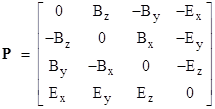
If we let x¹,x²,x³,x⁴ denote the coordinates x,y,z,t respectively, then equations (5a) and (5d) can be combined and expressed in the form

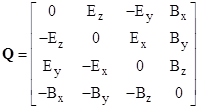
In exactly the same way we can combine equations (5b) and (5c) and express them in the form

where the matrix Q is an anti-symmetric matrix defined by

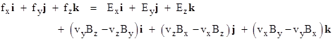
Returning again to equation (1a), we see that in the absence of a gravitational field the force on a particle with q = m = 1 and velocity v at a point in space where the electric and magnetic field vectors are E and B is given by

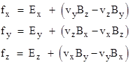
In component form this can be written as

Consequently the components of the acceleration are

Thus if the particle is stationary with respect to the original x,y,z,t coordinates, the force on the particle has the components

Now consider the same physical situation, but with respect to a system of inertial coordinates x′,y′,z′,t′ , aligned with the original coordinates, but moving in the positive x direction with speed v. Hence the components of the particle’s velocity in terms of these coordinates are v_x′ = –v and v_y = v_z = 0. For any given v there are constants K and k such that the components of the force parallel and perpendicular to x axis (respectively) are

Naturally the constants K and k both equal 1 at v = 0. From the preceding equations we see that the components of the electric field with respect to the primed and unprimed coordinate systems are related according to

By symmetry, replacing v with –v, we also have the reciprocal transformation

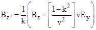
We've used the same K and k factors for both transformations, because to the first order we know k(v) is simply 1, implying that the dependence of k on v is of the second order, which suggests that K(v) and k(v) are even functions, i.e., K(v) = K(−v) and k(v) = k(−v). The two equations for the x components directly imply K = 1. Also, substituting the expression for E_y′ into the expression for E_y and solving the resulting equation for B_z′ gives

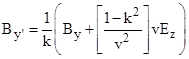
By the same token, substituting the expression for E_z′ into the expression for E_z and solving for B_y′ gives

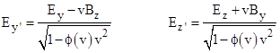
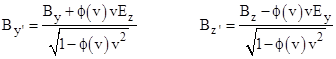
Therefore, letting ϕ(v) denote the quantity in square brackets for any given v, the general transformation equations for the electric and magnetic field components perpendicular to the velocity are

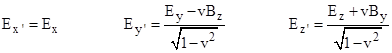
By analogous reasoning to that used in Section 1.7, we infer that ϕ(v) = 1, and hence

Therefore, from equation (9), we see that the transformed components of the total electromagnetic force are

It also follows that the components of the electric and magnetic field give the following invariants

Naturally the field components parallel to the velocity exhibit the corresponding invariance, i.e.,

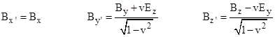
from which we infer the final transformation equation B_x′ = B_x. So, the complete set of transformation equations for the electric and magnetic field components from one system of inertial coordinates to another (with a relative velocity v in the positive x direction) is

Just as the Lorentz transformation for space and time intervals shows that those intervals are the components of a unified space-time interval, these transformation equations show that the electric and magnetic fields are components of a unified electro-magnetic field. The decomposition of the electromagnetic field into electric and magnetic components depends on the frame of reference. From the invariants noted above we see that, letting E² and B² denote squared magnitudes of the electric and magnetic field vectors at a given point, the quantity E² – B² is invariant (as is the dot product E×B), analogous to the invariant X² – T² for spacetime intervals. The combined electromagnetic field can be represented by the matrix P defined previously, which transforms as a tensor of rank 2 under Lorentz transformations. So too does the matrix Q, and since Maxwell's equations can be expressed in terms of P and Q (as shown by equations (8a) and (8b)), we see that Maxwell's equations are invariant under Lorentz transformations. Moreover, any physical force consistent with special relativity must transform in accord with (10), because otherwise a comparison of the forces in different frames of reference would give different results.

Return to Table of Contents