Appendices

1.  Vector Products

The dot and cross products are often introduced via trigonometric functions and/or matrix operations, but they also arise quite naturally from simple considerations of Pythagoras' theorem. Given two points a and b in the three-dimensional vector space with Cartesian coordinates (a_x,a_y,a_z) and (b_x,b_y,b_z) respectively, the squared distance between these two points is

If (and only if) these two vectors are perpendicular, the distance between them is the hypotenuse of a right triangle with edge lengths equal to the lengths of the two vectors, so we have

if and only if a and b are perpendicular. Equating these two expressions and canceling terms, we arrive at the necessary and sufficient condition for a and b to be perpendicular

This motivates the definition of the left hand quantity as the "dot product" (also called the scalar product) of the arbitrary vectors a = (a_x,a_y,a_z) and b = (b_x,b_y,b_z) as the scalar quantity

At the other extreme, suppose we seek an indicator of whether or not the vectors a and b are parallel. In any case we know the squared length of the vector sum of these two vectors is

We also know that S = |a| + |b| if and only if a and b are parallel, in which case we have

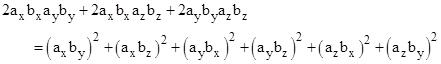
Equating these two expressions for S², canceling terms, and squaring both sides gives the necessary and sufficient condition for a and b to be parallel

Expanding these expressions and canceling terms, this becomes

Notice that we can gather terms and re-write this equality as

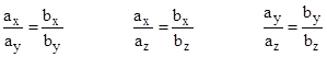
Obviously a sum of squares can equal zero only if each term is individually zero, which of course was to be expected, because two vectors are parallel if and only if their components are in the same proportions to each other, i.e.,

which represents the vanishing of the three terms in the previous expression. This motivates the definition of the cross product (also known as the vector product) of two vectors a = (a_x,a_y,a_z) and b = (b_x,b_y,b_z) as consisting of those three components, ordered symmetrically, so that each component is defined in terms of the other two components of the arguments, as follows

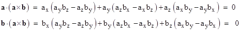
By construction, this vector is null if and only if a and b are parallel. Furthermore, notice that the dot products of this cross product and each of the vectors a and b are identically zero, i.e.,

As we saw previously, the dot product of two vectors is 0 if and only if the vectors are perpendicular, so this shows that a x b is perpendicular to both a and b. There is, however, an arbitrary choice of sign, which is conventionally resolved by the "right-hand rule". It can be shown that if θ is the angle between a and b, then a x b is a vector with magnitude |a||b|sin(θ) and direction perpendicular to both a and b, according to the right-hand rule. Similarly the scalar a×b equals |a||b|cos(θ).

2.  Total Derivatives

In Section 5.2 we gave an intuitive description of differentials such as dx and dy as incremental quantities, but strictly speaking the actual values of differentials are arbitrary, because only the ratios between them are significant. Differentials for functions of multiple variables are just a generalization of the usual definitions for functions of a single variable. For example, if we have z = f(x) then the differentials dz and dx are defined as arbitrary quantities whose ratio equals the derivative of f(x) with respect to x. Consequently we have dz/dx = f '(x) where f '(x) signifies the partial derivative ∂z/∂x, so we can express this in the form

In this case the partial derivative is identical to the total derivative, because this f is entirely a function of the single variable x.

If, now, we consider a differentiable function z = f(x,y) with two independent variables, we can expand this into a power series consisting of a sum of (perhaps infinitely many) terms of the form Ax^myⁿ. Since x and y are independent variables we can suppose they are each functions of a parameter t, so we can differentiate the power series term-by-term, with respect to t, and each term will contribute a quantity of the form

where, again, the differentials dx,dy,dz,dt are arbitrary variables whose ratios only are constrained by this relation. The coefficient of dy/dt is the partial derivative of Ax^myⁿ, with respect to y, and the coefficient of dx/dt is the partial with respect to x, and this will apply to every term of the series. So we can multiply through by dt to arrive at the result

The same approach can be applied to functions of arbitrarily many independent variables.

3. Differential Operators

The standard differential operators are commonly expressed as formal "vector products" involving the "del" symbol, which is defined as

where u_x, u_y, u_z are again unit vectors in the x,y,z directions. The scalar product of this “del” operator with an arbitrary vector field V is called the divergence of V, and is written explicitly as

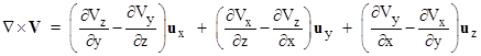
The vector product of “del” with an arbitrary vector field V is called the curl, given explicitly by

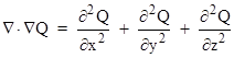
Note that the curl is applied to a vector field and returns a vector, whereas the divergence is applied to a vector field but returns a scalar. For completeness, we note that a scalar field Q(x,y,z) can be simply multiplied by the “del” operator to give a vector, called the gradient, as follows

Another common expression is the sum of the second derivatives of a scalar field with respect to the three directions, since this sum appears in the Laplace and Poisson equations. Using the "del" operator this can be expressed as the divergence of the gradient (or the "div grad") of the scalar field, as shown below.

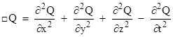
For convenience, this operation is often written as “del” squared, and is called the Laplacian operator. All the above operators apply to 3-vectors, but when dealing with 4-vectors in Minkowski spacetime the analog of the Laplacian operator is the d'Alembertian operator

4.  Tensor Differentiation

The easiest way to understand the motivation for the definitions of absolute and covariant differentiation is to begin by considering the derivative of a vector field A in three-dimensional Euclidean space. Such a vector can be expressed in either contravariant or covariant form as a linear combination of, respectively, the basis vectors u₁, u₂, u₃ or the dual basis vectors u¹, u², u³, as follows

where Aⁱ are the contravariant components and A_i are the covariant components of A, and the two sets of basis vectors satisfy the relations

where g_ij and g^ij are the covariant and contravariant metric tensors. The differential of A can be found by applying the chain rule to either of the two forms, as follows

If the basis vectors u_i and uⁱ have a constant direction relative to a fixed Cartesian frame, then du_i = duⁱ = 0, so the second term on the right vanishes, and we are left with the familiar differential of a vector as the differential of its components. However, if the basis vectors vary from place to place, the second term on the right is non-zero, so we must not neglect this term if we are to allow curvilinear coordinates.

As we saw in Part 2 of this Appendix, for any quantity Q = f(x) and coordinate xⁱ we have

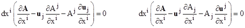
so we can substitute for the three differentials in (1) and re-arrange terms to write the resulting expressions as

Since these relations must hold for all possible combinations of dxⁱ , the quantities inside parentheses must vanish, so we have the following relations between partial derivatives

If we now let Aⁱ_;j and A_i;j denote the projections of the ith components of (2a) and (2b) respectively onto the jth basis vector, we have

and it can be verified that these are the components of second-order tensors of the types indicated by their indices (superscripts being contravariant indices and subscripts being covariant indices). If we multiply through (using the dot product) each term of (2a) by uⁱ, and each term of (2b) by u_i, and recall that uⁱu_j = dⁱ_j, we have

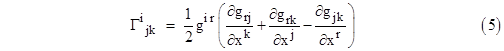
For convenience we now define the three-index symbol

which is called the Christoffel symbol of the second kind. Although the Christoffel symbol is not a tensor, it is very useful for expressing results on a metrical manifold with a given system of coordinates. We also note that since the components of u_i×u^j are constants (either 0 or 1), it follows that ∂(u_i×u^j)/∂x^k = 0, and expanding this partial derivative by the chain rule we find that

Therefore, equations (3) can be written in terms of the Christoffel symbol as

These are the covariant derivatives of, respectively, the contravariant and covariant forms of the vector A with respect to the coordinate x^k. Obviously if the basis vectors are constant (as in Cartesian or oblique coordinate systems) the Christoffel symbols vanish, and we are left with just the first terms on the right sides of these equations. The second terms are needed only to account for the change in basis with position of general curvilinear coordinates.

It might seem that these definitions of covariant differentiation depend on the fact that we worked in a fixed Euclidean space, which enabled us to assign absolute meaning to the components of the basis vectors in terms of an underlying Cartesian coordinate system. However, it can be shown that the Christoffel symbols we've used here are the same as the ones defined in Section 5.4 in the derivation of the extremal (geodesic) paths on a curved manifold, wholly in terms of the intrinsic metric coefficients g_ij and their partial derivatives with respect to the general coordinates on the manifold. This should not be surprising, considering that the definition of the Christoffel symbols given above was in terms of the basis vectors u_j and their derivatives with respect to the general coordinates, and noting that the metric tensor is just g_ij = u_i×u_j . Thus, with a bit of algebra we can show that

in agreement with Section 5.4. We regard equations (4) as the appropriate generalization of differentiation on an arbitrary Riemannian manifold essentially by formal analogy with the flat manifold case, by the fact that applying this operation to a tensor yields another tensor, and perhaps most importantly by the fact that in conjunction with the developments of Section 5.4 we find that the extremal metrical path (i.e., the geodesic path) between two points is given by using this definition of "parallel transport" of a vector pointed in the direction of the path, so the geodesic paths are locally "straight".

Of course, when we allow curved manifolds, some new phenomena arise. On a flat manifold the metric components may vary from place to place, but we can still determine that the manifold is flat, by means of the Riemann curvature tensor described in Section 5.7. One consequence of flatness, obvious from the above derivation, is that if a vector is transported parallel to itself around a closed path, it assumes its original orientation when it returns to its original location. However, if the metric coefficients vary in such a way that the Riemann curvature tensor is non-zero, then in general a vector that has been transported parallel to itself around a closed loop will undergo a change in orientation. Indeed, Gauss showed that the amount of deflection experienced by a vector as a result of being parallel-transported around a closed loop in a two-dimensional manifold is exactly proportional to the integral of the curvature over the enclosed region.

The above definition of covariant differentiation immediately generalizes to tensors of any order. In general, the covariant derivative of a mixed tensor T consists of the ordinary partial derivative of the tensor itself with respect to the coordinates x^k, plus a term involving a Christoffel symbol for each contravariant index of T, minus a term involving a Christoffel symbol for each covariant index of T. For example, if r is a contravariant index and s is a covariant index, we have

It's convenient to remember that each Christoffel symbol in this expression has the index of x^k in one of its lower positions, and also that the relevant index from T is carried by the corresponding Christoffel symbol at the same level (upper or lower), and the remaining index of the Christoffel symbol is a dummy that matches with the relevant index position in T.

One very important result involving the covariant derivative is known as Ricci's Theorem. The covariant derivative of the metric tensor is g_ij is

If we substitute for the Christoffel symbols from equation (5), and recall that

we find that all the terms cancel out and we're left with g_ij;k = 0. Thus the covariant derivative of the metric tensor is identically zero, which is what prompted Einstein to identify it with the gravitational potential, whose divergence vanishes, as discussed in Section 5.8.

5. Variational Principle for the Gravitational Field

In Section 5.4 we described the variational approach to deriving equations of motion, by finding the path along which a particle can travel between two given events such that the integral of a certain function (sometimes called the “action”) along that path is stationary, i.e., unaffected by any incremental deviations from that path, provided the variations are zero at the endpoints of the path. The very same approach can be taken to deriving the equations of a field, by finding the values of the field variables within any region enclosed by a given boundary such that the integral of a certain function within that region is stationary, i.e., unaffected by any incremental deviations from those values, provided the variations are zero on the boundary.

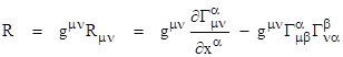
One advantage of the variational approach is that the stationarity of the field variables automatically implies that the field satisfies certain conservation laws. In his paper of November 4, 1915, Einstein showed that his proposed gravitational field equations for the vacuum satisfy the conservation of energy and momentum by showing that they can be derived using the variational principle with a suitable function which Einstein called the “Hamiltonian function”. As explained in Section 5.8, the vacuum field equations are R_μn = 0 where R_μn is the Ricci tensor, which, if we impose the coordinate condition (−g)^1/2 = 1, is given by equation (7) of that section. Perhaps the most natural function to take as the Hamiltonian is the Ricci scalar

However, Einstein takes only the second term (with positive sign). This may seem surprising, but it can be shown that the integral of the first term (involving the derivative of the Christoffel symbol) throughout the region of interest can be expressed as a surface integral on the boundary (Green’s theorem), and since we stipulate that the variation is zero on the boundary, this contributes nothing to the variation of the integral of R over that region. Therefore, instead of using R as the Hamiltonian, Einstein gets the same result by taking as the Hamiltonian of the gravitational field the function

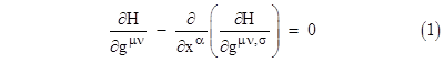
We require that the integral of this scalar function within the region of interest be stationary for any incremental variations in the field variables, with the stipulation that the variations vanish at the boundary of the region. Taking H as a function of the g^μν and their derivatives g^μν,σ = dg^μν/dx^σ, the variational method described in Section 5.4 leads to Euler’s equations

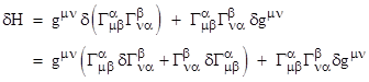
We wish to show that this represents the vacuum field equations. By the product rule, the differential of H is

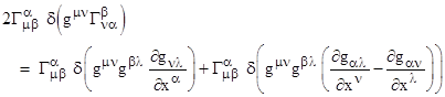
The two terms in parentheses are equal (as can be seen by swapping α and β), so this can be written as

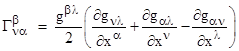
From the definition of the Christoffel symbol we have

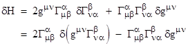
so the first term in the preceding expression can be written as

The second term vanishes (because we negate the entire term if we transpose μ with β and λ with ν), so the differential of H can be written as

To simplify the expression in parentheses, note that we can differentiate the identity g_νλg^βλ = δ^β_ν (where δ^β_ν = 0 if β¹ν and δ^β_ν = 1 if β=ν) with respect to x^α by the product rule to give

Multiplying both sides by g^μν we get

Solving these equations for the partials of g^μσ with respect to x^α, we get the relation

Letting g^μβ,σ denote the partial on the left side, we can substitute this for the quantity in parentheses in the equation for the differential of the Hamiltonian to give

Therefore we have the partial derivatives

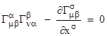
Substituting into the Euler equations (1), this gives

in agreement with the vacuum field equations given by equation (7) in Section 5.8.

6. Geodesic Redundancy

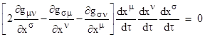
As noted in Section 6.2, we apparently made use of only two of the three geodesic equations, excluding equation (8), when deriving the relativistic orbital precession. Recall that we integrated equations (7) and (9), and then substituted the results into the line element, which then gave the equation of motion represented by (10). To show that this is consistent with the remaining geodesic equation (8), we can differentiate equation (10) with respect to τ and divide through by 2(dr/dτ) to give

This is the same equation we would get if we inserted the squared derivatives of the coordinates into equation (8). Thus we have consistency with all of the geodesic equations.

In general, if a path satisfies all but one of the geodesic equations, the metric line element ensures that it satisfies the remaining geodesic equation as well. To show this, we can write the general metric in the form

and differentiate with respect to τ to give

For the total derivatives of the metric coefficients we can make the substitutions

so we have

Also, since the dummy indices in the two terms are independent, we can replace μ and n in the first term with σ and ω, and divide through by 2, to give the equivalent form

The expression inside the square brackets is similar to one form of the geodesic equations of the surface, but not exactly the same. However, notice that we have the identity

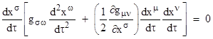
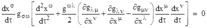
This identity can be directly verified by noting first that the expression in square brackets vanishes trivially if all the indices are equal, and then noticing that the combined coefficient of a given product of three derivatives vanishes if two indices are equal and one is different, and finally noticing that the combined coefficient of each product vanishes over the six permutations of all distinct indices. So, we can subtract half of this identically vanishing expression from the previous equation and factor out g_σω to give the result

The expressions inside the square brackets for ω = 0,1,2,3 represent the four geodesic equations, whose vanishing is the necessary and sufficient condition for a path to be stationary (see Section 5.4). Thus if any three of the geodesic equations are satisfied, then the fourth is automatically satisfied by virtue of the metric.

7.  Independent Components of the Curvature Tensor

As shown in Section 5.7, the fully covariant Riemann curvature tensor at the origin of Riemann normal coordinates, or more generally in terms of any “tangent” coordinate system with respect to which the first derivatives of the metric coefficients are zero, has the symmetries

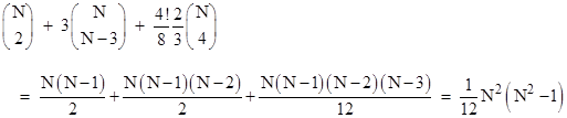
These symmetries imply that although the curvature tensor in four dimensions has 256 components, there are only 20 algebraic degrees of freedom. To prove this, we first note that the anti-symmetry in the first two indices and in the last two indices implies that all the components of the form R_aaaa, R_aabb, R_aabc, R_abcc, and all permutations of R_aaab are zero, because they equal the negation of themselves when we transpose either the first two or the last two indices. The only remaining components with fewer than three distinct indices are of the form R_abab and R_abba, but these are the negatives of each other by transposition of the last two indices, so we have only six independent components of this form (which is the number of ways of choosing two of four indices). The only non-zero components with exactly three distinct indices are of the forms R_abac = –R_baac = –R_abca = R_baca, so we have twelve independent components of this form (because there are four choices for the excluded index, and then three choices for the repeated index). The remaining components have four distinct indices, but each component with a given permutation of indices actually determines the values of eight components because of the three symmetries and anti-symmetries of order two. Thus, on the basis of these three symmetries there are only 24/8 = 3 independent components of this form, which may be represented by the three components R₁₂₃₄, R₁₃₄₂, and R₁₄₃₂. However, the skew symmetry implies that these three components sum to zero, so they represent only two degrees of freedom. Hence we can fully specify the Riemann curvature tensor (with respect to “tangent” coordinates) by giving the values of the six components of the form R_abab, the twelve components of the form R_abac, and the values of R₁₂₃₄ and R₁₃₄₂, which implies that the curvature tensor (with respect to any coordinate system) has 6 + 12 + 2 = 20 algebraic degrees of freedom.

The same reasoning can be applied in any number of dimensions. For a manifold of N dimensions, the number of independent non-zero curvature components with just two distinct indices is equal to the number of ways of choosing 2 out of N indices. Also, the number of independent non-zero curvature components with 3 distinct indices is equal to the number of ways of choosing the N–3 excluded indices out of N indices, multiplied by 3 for the number of choices of the repeated index. This leaves the components with 4 distinct indices, of which there are 4! times the number of ways of choosing 4 of N indices, but again each of these represents 8 components because of the symmetries and anti-symmetries. Also, these components can be arranged in sets of three that satisfy the three-way skew symmetry, so the number of independent components of this form is reduced by a factor of 2/3. Therefore, the total number of algebraically independent components of the curvature tensor in N dimensions is

Return to Table of Contents