Shapiro Time Delay

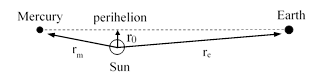
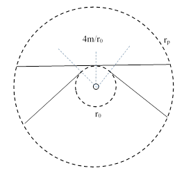
Suppose a radar pulse is emitted from Earth and just grazes past the Sun, striking the planet Mercury on the opposite side (during a superior conjunction), and then returns to Earth, as depicted schematically in the figure below (not to scale), where r_e and r_m are the distances from the Sun to Earth and Mercury respectively, and r₀ is the distance from the Sun’s center to the point of closest approach (perihelion) of the light path.

In 1964 Irwin Shapiro pointed out that the timing of such radar signals could provide a “fourth test” of general relativity (in addition to the original three proposed by Einstein: gravitational redshift, light deflection, and the precession of orbits). Shapiro noted that, according to general relativity, the radar returns should be slightly delayed as a result of passing through the Sun’s gravitational field.

As a practical matter, only the variation in the transit time as the perihelion distance changes (e.g., as the planet approaches superior conjunction) can be measured, but in theory we can evaluate the absolute transit time given the spatial distances in terms of suitable coordinates. However, a survey of the literature shows a wide variety of at least formally distinct predictions for the precise amount of delay, based on a variety of solutions methods. There are three main sources of variation. First, some authors work in terms of Schwarzschild coordinates while others work in terms of isotropic coordinates. Second, some authors express their results in terms of coordinate time, whereas others apply corrections to account for the gravitational time dilation and/or the motion of the clock on Earth. Third, some authors assume a “straight path” approximation whereas others use the actual (curved) null geodesic path.

The first two of these are fairly straight-forward differences that are easily reconciled, but the third – involving the use of a “straight” path versus the geodesic path – is actually somewhat subtle, and there are many erroneous claims in the literature that the “straight” path approximation makes no difference in the result to the first order in m/r. Surprisingly, it actually does make a first-order difference (as explained below), and the failure to correctly account for this is responsible for much confusion on this topic.

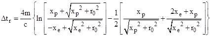
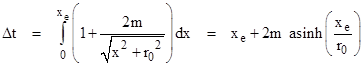
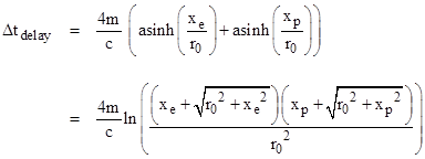
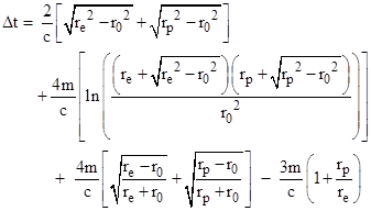
In his original paper Shapiro presented, without derivation, the following equation (with slight notational differences) for the relativistic delay in the round-trip transit time:

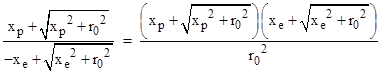
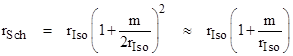
where m is the mass of the Sun in geometrical units, and he identifies x_e as the distance “along the line of flight” between the Earth and the perihelion, and x_p as the distance between the target planet (e.g., Mercury) and the perihelion. He says he is using Schwarzschild coordinates, and it’s clear that he is using the “straight path” approximation, and is correcting for the effect of the Sun’s gravity (but not the Earth’s motion) on the Earth clock, as we will confirm below. Making use of the algebraic identity

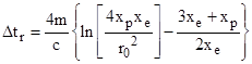
he noted that in the limit as x_p and x_e are much greater than r₀ the expression for the delay reduces to

For observational purposes the logarithmic term is most significant, since it gives the variation in the transit time as r₀ changes, and it turns out that this term is insensitive to all the variations and discrepancies between the published results. However, to the extent that the other terms matter, we will see that they are not exactly correct.

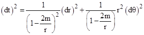
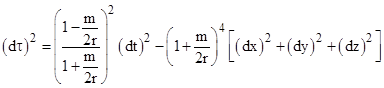
First we will show how Shapiro’s formula can be derived from the premises he stated, i.e., a “straight path” in terms of Schwarzschild coordinates. For convenience we use polar Schwarzschild coordinates, in terms of which we have the metric relation for null paths

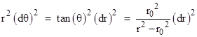
A straight line path with closest approach to the Sun of r₀ is given by r sin(θ) = r₀. Thus we have r cos(θ)dθ + dr sin(θ) = 0, so

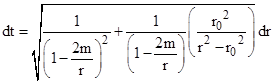
Substituting into the metric and taking the square root, this gives

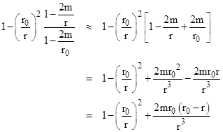
To the first order in m/r this is equivalent to

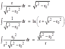
Making use of the elementary integrals

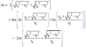
we get for the round trip from Earth to planet and back

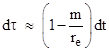
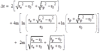
Bearing in mind that Shapiro expressed his formula in terms of the x coordinate where r² = x² + r₀², we see that the first term is just his “Newtonian” transit time 2(x_e + x_p) and the next two terms agree with Shapiro’s formula except that, in the square brackets of the last term, we have x_e/r_e + x_p/r_p whereas his formula has x_p/r_p + (2x_e + x_p)/r_e. The difference is due to the fact that the overall transit time as measured by a clock on the Earth is also affected by time dilation due to the Sun’s gravitational field.  (A clock on Earth is also affected by the Earth’s gravitational field, but this is a negligibly small effect by comparison.) Since a clock at the Earth’s orbit runs slow compared with coordinate time, the transit delay for the light pulse appears to be less, i.e., the measured amount of delay is reduced. For a stationary point at radial coordinate r_e we have

and since the overall transit time is approximately 2(x_e + x_p) it follows that the measured delay in terms of a clock on Earth is reduced by 2m(x_e + x_p) /r_e. Including this (subtractive) term, we get Shapiro’s formula exactly.

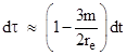
Now, this derivation can be criticized on three grounds. First, the use of Schwarzschild coordinates may be misleading because the elements of planetary orbits in astronomy are ordinarily quoted in terms of isotropic coordinates, which use a radial coordinate that differs to the first order from the Schwarzschild radial coordinate (as discussed below). Second, although a correction for the time dilation due to the Sun’s gravity was included, the comparable correction for the Earth’s orbital velocity was omitted. As discussed in another note, for a circular orbit the combined effect of gravitational potential and orbital velocity yields the time dilation

Since the overall transit time is approximately 2(x_e + x_p) the measured delay in terms of a clock on Earth is actually reduced by (3m/r_e)(x_e + x_p). Third, and most importantly, the “straight path” approximation is actually erroneous in the first order, contrary to many claims in the literature (as discussed below).

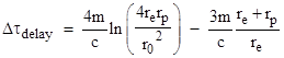
The corrections for time dilation of Earth clocks are constant effects and can be handled separately, so for this remainder of this note we will focus mainly on the coordinate time delays, noting that both the Schwarzschild and isotropic coordinate systems use the same time coordinate. In the limit of small r₀ compared with r_e and r_p (so the r and x coordinates are essentially equal) the second and third terms (which are regarded as the non-Newtonian “extra” delay) of Shapiro’s formula (omitting the clock correction) reduce to

where we have divided by c to convert to units of seconds. For example, the mean orbital radii of the Earth and Mercury are (150)10⁹ meters and (55)10⁹ meters respectively, and the radius of the Sun is (6.95)10⁸ meters, and the mass of the Sun (in geometric units) is 1475 meters, and the speed of light is (3)10⁸ m/sec, so equation (1) gives a time delay of 199 μsec for a pulse just grazing the Sun. If the time dilation effects for Earth clocks were included, this would be reduced to about 180 μsec. However, if the orbital elements are actually expressed in terms of isotropic coordinates, we need to correct for the difference between the definitions of the radial coordinates, which are related by

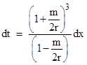
The x and y coordinates for these two systems are scaled accordingly. Recall that the nominal transit time is 2(x_e + x_p)/c. Replacing x_e with (1+m/x_e)x_e = x_e + m, and similarly for x_p, the difference amounts to about 4m/c. Thus the –1 term inside the square brackets of equation (1) should be removed. To confirm this, we will derive the time delay in terms of isotropic coordinates, in which the speed of light at any given point is the same in all directions. For the moment we will continue to use the “straight path” approximation, although now the straightness is in terms of isotropic coordinates. In these coordinates the Schwarzschild metric takes the form

where r² = x² + y² + z². For a pulse of light moving in the purely x direction this implies

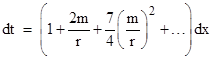
Expanding to a series in powers of m/(2r), we have

Neglecting the second and higher order terms, we can integrate this from the Earth to the perigee of the path (closest to the Sun) to give the elapsed time (in units of meters)

(Incidentally, people sometimes mistakenly think this integral is of the inverse speed in terms of Schwarzschild coordinates, in which the radial speed of light is 1 – 2m/r to the first order, and they imagine that this analysis is overlooking that the path has a tangential component for which the speed of light is 1 – m/r. But, as noted, this derivation is in terms of isotropic coordinates, in which the speed of light is isotropic, so the tangential part of the path is not neglected. See Appendix 1 for a derivation explicitly based on integrating the inverse speed in Schwarzschild coordinates.) The last term on the right side represents the relativistic delay. A similar expression gives the elapsed time between perigee and the target planet, and we can add the delay terms together and multiply by 2 (and divide by c to convert to units of seconds) to give the total round-trip delay

Naturally the time delay is most noticeable when the light pulse passes very close to the Sun, meaning that r₀ is very small (on the order of the Sun’s radius) in comparison with the orbital radii of the planets. In that case the square roots in the above expression for the coordinate time delay are approximately equal to r_e and r_p respectively, so we can write it as

As expected, this exceeds equation (1) by 4m/c. Thus for the same values of the parameters (interpreted now in terms of isotropic coordinates) this gives the coordinate time delay of 219 μsec for a pulse just grazing the Sun. If we include the time dilation effects of the Sun’s gravity and the Earth’s motion on Earth based clock as described above we get

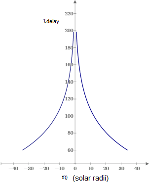
This reduces the delay time (for a grazing pulse between Earth and Mercury) to 199 μsec. (This is not to be confused with the previous value of 199 μsec because that was uncorrected, and it just so happens that the orbital radii of Earth and Mercury give (r_e + r_p)/r_e = 4/3, so the coordinate effects and the full time dilation effects are roughly equal.) A plot of this time delay as a function of r₀ is shown below.

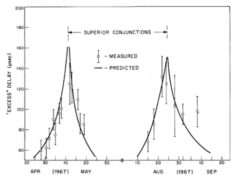
The curve asymptotically approaches the baseline time dilation effect as r₀ increases. During the superior conjunctions that Shapiro actually observed in 1967, Mercury did not pass directly behind the Sun, so the smallest perihelion value was actually several solar radii. As a result, the predicted time delays were somewhat lower than the peak value corresponding to a Sun-grazing path. It should also be noted that identifying the non-Newtonian delay is somewhat arbitrary, since Newtonian theory doesn’t make a clear prediction for how light behaves in a gravitational field, and it is even problematic to define the Newtonian distance in this scenario. Furthermore, it isn’t feasible to determine the orbital radii to the level of precision corresponding to 200 μsec, other than by radar ranging itself. Hence, only the variations in the delays (the shape of the curve) as the perihelion distance changes are actually detectable. A reproduction of Shapiro’s plot from his 1968 paper presenting observational results for Mercury at two superior conjunctions in 1967 is shown below.

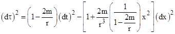
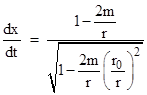
Up to this point the derivations have been based on the coordinate-dependent “straight path” approximation. A more rigorous derivation, that does not rely on this approximation, can be based on the exact equation of motion for a light pulse in a gravitational field. As discussed in another note, the equation of motion in terms of Schwarzschild coordinates is

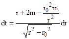
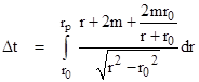
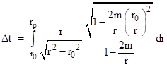
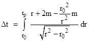
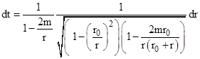
where r₀ is the perihelion radius. If we write 2m/r₀ as (2m/r)(r/r₀) and expand this to the first order in m/r (see Appendix 2) we arrive at the integral for the coordinate time required for the pulse to travel between perihelion and planet

It’s worth noting that we could have decomposed the numerator in different ways, such as r + 3m – mr/(r + r₀), but the latter term has a very complicated compound integral, so it’s best to use the form above. Making use of two of the simple integrals noted previously along with

we have the two-way coordinate time interval (in geometric units) from one planet to the other and back

The first term corresponds to the Newtonian interval 2(x_e + x_p) as in our previous solution, and the second term matches the delay time from our previous solution. However, the third term was not present in the previous solutions. In the limit of small r₀ the third term is just 4m, so the coordinate delay time (for Schwarzschild coordinates in units of seconds) is

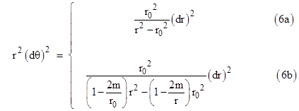
For a Sun-grazing pulse between Earth and Mercury (round trip) this yields a coordinate delay time of 239 μsec, compared with only 199 μsec given by equation (1). This is a difference of 8m/c, even though both are expressed in terms of Schwarzschild coordinates. The only difference is that (1) was based on the “straight path” approximation” and (2) was based on the actual geodesic path. The relations between dr and dθ for a (Schwarzschild) “straight” path and the actual null geodesic path (all in terms of Schwarzschild coordinates) are

If we substitute the “straight” path relation (6a) into the Schwarzschild metric and integrate we get the time delay given by (1), but if we substitute the actual null geodesic path relation (6b) into the Schwarzschild metric and integrate we get the time delay given by (3). Based on many statements in the literature, this is an impossible outcome, because the authors assure us that the straight path and the geodesic path can differ only in the second order. For example, Misner, et al, state that

The lapse of coordinate time between transmission of the radar beam and reflection at the detector is the same for a straight path in the [first order] coordinates as for the slightly curved path which the beam actually follows. The two differ by only a fractional amount proportional to the angle of deflection squared, which is far from discernable.

Along with this they present a drawing that shows a smoothly curving path over the whole range from Earth to planet, for which the path length would indeed differ from a straight line only by an amount proportional to the square of the deflection angle. Likewise D’Inverno justifies the use of the straight path approximation by saying it gives the same result as the actual path to the first order, and Ohanian & Ruffini echo Misner, saying

Of course, because of the deflection of the path of light, will not be exactly straight. But this has next to no effect on the travel time because the difference in length between the straight and curved paths shown in Figure 4.8 is only of order θ² where θ is the deflection angle; this difference is therefore a second-order correction which we can ignore.

Again their figure shows a path curving smoothly over the entire range between planets. Similar justifications appear in many other references. It certainly sounds plausible, especially in view of the figures, since they suggest that the different paths would be related as the cosine of the small angle between them, and the cosine differs from 1 by only θ²/2. But how then do we explain the difference of 8m/c in the elapsed coordinate times between the straight and geodesic solutions?

To see whether this might be some artifact of the Schwarzschild coordinates (which are not conformal), we can determine the solution for the actual null geodesic path in terms of isotropic coordinates and compare with the result for isotropic coordinates with the straight path approximation given by (2). In another note we determined that the equation of motion for a pulse of light in isotropic coordinates is

Replacing m/r₀ with (m/r)(r/r₀) and expanding in powers of m/r, we arrive at the coordinate time for the transit from perihelion to a planet (for isotropic coordinates)

We note again that the terms in the numerator involving m can be partitioned in various ways, so we choose the way that leads to simple closed form integrals. This result is formally identical to the expression for the geodesic path in Schwarzschild coordinates, except that the coefficient of the last term in the numerator is 2 instead of 1. As a result, the expression for the delay time (defined again as the overall transit time minus the first term) in units of seconds in the limit of small r₀ is

Thus we find once again that the time delay for the geodesic path exceeds that based on the straight path approximation by 8m/c. (This difference seems not only too large, but in the wrong direction, since Fermat’s principle of least time, applicable since the metric coefficients are independent of the coordinate time, implies that the geodesic path minimizes the elapsed coordinate time – for a given initial trajectory between two fixed points. However, those conditions don’t apply here.) In fact, it isn’t just the elapsed time. Integrating the spatial lengths of the straight and geodesic paths shows the same first order difference, so the claims that the path lengths differ only in the second order are incorrect… but how can this be?

The answer is interesting. People have been misled by the drawings that show a smooth bow shape for the geodesic path, as if the path is gradually curved all along its length. If that were accurate, the lengths would indeed differ only in the second or higher order of the deflection angle. But in fact the path consists of two virtually straight legs, with almost all of the angular deflection occurring very near the perihelion. This is shown (in exaggerated form) in the figure below.

The straight (horizontal) path consists of two segments extending from the point of tangency on the r₀ circle to the r_p circle. The geodesic path also has two segments of that same length, extending from tangent points on the r₀ circle out to the r_p circle, but in addition the path has the circular arc segment at the radius r₀ (approximately) through the relativistic deflection angle of 4m/r₀. Hence the length of that arc segment is 4m, and it is traversed twice for the round trip, which yields the extra delay time of 8m/c.

Of the texts I’ve seen, very few give derivations based on the actual geodesic path (exceptions being Weinberg and Wald), and none of them note (let alone try to reconcile) the difference between the geodesic results and those based on the straight path approximation. The discrepancy does, however, seem to have vaguely troubled various authors. For example, one online source presents the formula (1) based on the straight path in Schwarzschild coordinates, without the time dilation corrections, and computes a delay of 160 μsec for Venus with a particular r₀. They note that the actual measured value was 180 μsec, so they acknowledge that their computed value was low by 4m/c. Had they applied the time dilation correction they would have been low by about 8m/c. They justify not applying the correction by saying “the correction affects only the eight decimal place and can therefore be omitted” (luckily, since it would double their error), and they waive off the remaining discrepancy by saying “The difference indicates that my value of r₀ [acquired from an astronomical program for the precise date of the observation] was slightly too big”. Had they used the correct formula and applied the appropriate corrections, there would have been no discrepancy.

In summary, assuming the orbital radii are expressed in terms of isotropic coordinates (most common for astronomical work), and taking into account the geodesic path and the corrections for time dilation of the Earth-based clock due to both the Sun’s gravity and the Earth’s motion, the actual time delay (in units of seconds, to the first order in m/r) is

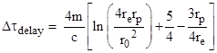
One might think that we are justified in regarding the first term as the baseline flat spacetime prediction, since it is the term that remains if we set m = 0 (no gravity), but there is a subtlety because the initial trajectory angle compatible with given values of the radii varies with m. Nevertheless, it’s conventional to hold the radii fixed and let the initial trajectory vary.  In the limit of small r₀, the baseline term is just 2(r_e + r_p) and the extra delay terms proportional to m reduce to

For the planet Mercury the ratio r_p/r_e is about 1/3, so the last two terms in the square brackets reduce to approximately +1. Hence the delay, in terms of proper time on the Earth for a radar pulse just grazing the Sun to go to Mercury and back is about 238 μsec, and for a pulse with perihelion of about 4 solar radii it predicts 183 μsec, compared with the reported measurement of 180 μsec. Mercury’s orbit is actually fairly elliptical, so it’s distance from the Sun varies significantly from the average. Hence the agreement within 3 μsec for this simplistic formula using the average radii is surprisingly good. For the planet Venus, with an orbital radius of (108)10⁹ meters, the formula predicts a maximum delay for a pulse grazing the Sun of about 246 μsec.

Appendix 1

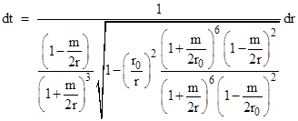
A simplistic derivation based on integrating the speed along a (assumed linear) path is sometimes appealing to students. Is isotropic coordinates this is straight-forward, since the speed of light is isotropic, but in Schwarzschild coordinates we need to take into account the directional dependence of light speed. As discussed elsewhere, the speed is 1 – 2m/r in the radiaql direction and 1 – m/r in the tangential direction. For constant y and z the Schwarzschild metric can be written as

where r² = x² + y². For a light pulse we  have dτ = 0 and the speed of a pulse moving along a line of constant y = r₀ is

This confirms that the tangential speed (to the first order) when r = r₀ is 1 – m/r and the radial speed when r is much greater than r₀ is 1 – 2m/r. Noting that dx = (r/x)dr, we can write the elapsed coordinate time from r₀ to r_p as the integral

Expanding the integrand to the first order in m, this can be written as

which, as expected, is the same integral as in our previously derivation based on the straight path approximation in Schwarzschild coordinates.

Appendix 2

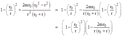
To the first order, the expression under the square root in equation (3) can be written as

Multiplying the numerator and denominator of the last term on the right by (r₀ + r), this becomes

With this the equation of motion can be written as

Now we can apply the binomial expansion to arrive at the integrand of equation (4).

Return to MathPages Main Menu