The Zeta Function

It is very probable that all roots are real. Of course one would wish for a rigorous proof here; I have for the time being, after some fleeting vain attempts, provisionally put aside the search for this, as it appears dispensable for the immediate objective of my investigation.

                                                                                                        Riemann, 1859

One of the simplest infinite series is the so-called harmonic series, which is the sum of the reciprocals of the natural numbers

Although this series grows very slowly as we add each successive term, it eventually exceeds any finite limit value. To see this, note that 1/3 + 1/4 is greater than 1/4 + 1/4, so the sum of the former two terms exceeds 1/2. Also, each of the next four terms, 1/5 through 1/8, is greater than or equal to 1/8, so those four terms contribute more than 1/2 to the total. Likewise each of the next eight terms, from 1/9 through 1/16, is greater than or equal to 1/16, so those eight terms contribute more than 1/2 to the total. And so on. This shows that we increase the sum by more than 1/2 each time we double the number of terms, so the sum has no finite upper bound.

In the late 17^th century several mathematicians went on to consider the sum of the reciprocals of the squares of the natural numbers, as shown below.

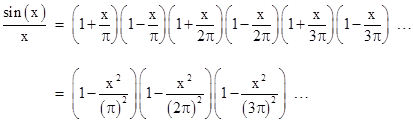
After lengthy calculations and analysis, Jakob Bernoulli in 1689 concluded that this series converges on a value less than 2, but it converges so slowly that it is difficult to determine the value with any precision by manual calculations. (Even with modern computers it requires thousands of terms to achieve the convergence of the first few digits.) However, in 1735, Leonard Euler found an elegant expression for the exact value of this summation. By then it was well known that the function sin(x)/x has the power series expansion

The roots of this function are simply the values –π, +π, –2π, +2π, –3π, +3π, … and so on. Therefore, Euler reasoned (by analogy with finite polynomials), we can express this function as the product of linear factors

Multiplying these factors (again by analogy with finite polynomials), we get an expression of the form

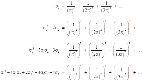
where the coefficients σ_j are the elementary symmetric functions (i.e., the sum of all products of j elements) of the squared reciprocal roots. Using Newton’s identities, this immediately gives

and so on. Now, equating the coefficients in equations (1) and (2), we have

Making these substitutions into the preceding equations and simplifying, Euler arrives at the results

and so on. For convenience, we define the zeta function as follows:

This is just a partial definition, since it defines ζ(s) only for values of s for which the infinite series converges, which happens to be when the real part of s is greater than 1. Later we will consider whether there is a natural way to extend the definition of ζ(s) to other values of s, for which the series does not converge.

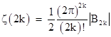
Extending the above results to any positive even power, we see that ζ(2k) is given by

where B_j are the Bernoulli numbers, B₀ = 1, B₁ = –1/2, B₂ = 1/6, B₃ = 0, B₄ = –1/30, B₅ = 0, and so on.

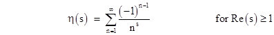
We now introduce a function that is identical to ζ(s), except with alternating the signs of the terms, i.e.,

This (again) is just a partial definition, since it applies only to values of s for which the series converges. However, in this case, the series converges for s = 1, because we have

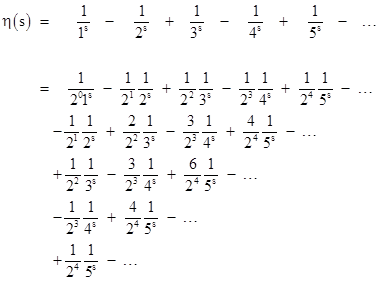
which follows directly from the series expansion of the natural logarithm. Because the terms of η(s) have alternating signs, we can easily apply the technique of analytic continuation by exploiting conditional convergence based on a suitable partitioning of the terms. To be precise, we can expand this function into a two-dimensional array whose rows converge to finite values, and such that the sum of those finite values also converges on a finite value. This can be done as follows:

Each term of the original series is partitioned into the terms of a diagonal of the array, with binomial coefficients. Although the original sequence of partial sums converges only for s with Re(s) ≥1, the rows of the partitioned expression converge for any complex value of s, and the sum of those row sums also converges. Thus, summing the rows and the columns, we can give a complete definition of the η function as

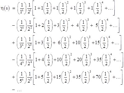
An equivalent but more rapidly converging expression can be inferred from the partitioning shown below.

The series in square brackets on the nth row sums to 2ⁿ, so it cancels with the leading factor of 1/2ⁿ. In this case, if we sum orthogonally (i.e., each row first, and then the column), we get back the original terms of the η function, but if we sum the diagonals we get a convergent value. (Compare this with the previous case, in which the diagonals represented the original divergent terms, and we get a convergent value by summing orthogonally.) Evaluating the sum by diagonals, and noting that each term in any given diagonal has the same powers of 2 in the denominator, we get the expression

Using this we can compute unambiguous values of η(s) for any complex value of s. For example, we find η(–2k) = 0 for all positive integers k, and η(0) = 1/2, η(–1) = 1/4, η(–3) = –1/8, η(–5) = 1/4, η(–7) = –17/16, and so on.

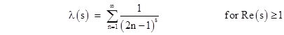
We were able to directly define a unique finite expression for the value of the η(s) for all s because it is an alternating series which is conditionally convergent for suitable dissections arrangements of the terms, but this technique doesn’t apply as easily to ζ(s), which has all positive terms. To establish the relationship between these two functions it’s convenient to first define a function λ(s) (in the region of convergence) as the sum of just the odd terms of the zeta function, i.e.,

Now we observe that (at least within the range of convergence) the series expressions for ζ(s) and η(s) can both be expressed as the sum or difference of two interlaced series as follows:

From these we get the relations

These relations are certainly valid for all values of s for which the series converge, and the left-hand relation is a well-behaved analytic function for all values of s other than s = 1, so we can say that it holds good for the entire functions by analytic continuation. Therefore, making use of (4), we have an expression for the zeta function that converges for all s (except s = 1):

We have ζ(–2k) = 0 for every positive integer k. These are called the trivial roots of the zeta function. Other notable values are ζ(0) = –1/2, ζ(–1) = –1/12, and ζ(1–2k) = –B_2k/(2k). In addition to the trivial roots, there also exist complex roots, and Riemann famously hypothesized that they are all of the form

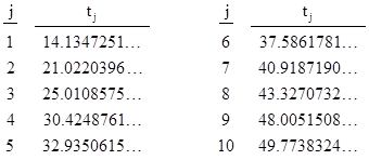
for real t. Using (5), we find that the first ten non-trivial roots of the Riemann zeta function have the values of t shown below.

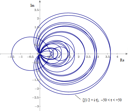
A plot of the values of ζ(1/2 + it) for t ranging from –50 to +50 is shown below.

The roots occur each time the locus passes through the origin.

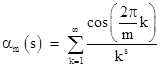
A key step in the preceding discussion was to consider the series with alternating signs, which we represented by multiplying the kth term by (–1)^k, but we could equivalently have multiplied each term by cos(kπ). This leads us to consider a generalized family of functions given by

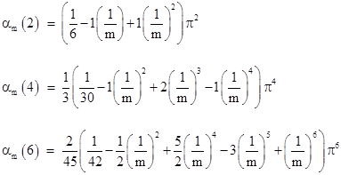
Clearly we have ζ(s) = α₁(s) and η(s) = α₂(s). We find the interesting results

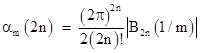
Recognizing the Bernoulli polynomials B_2j(x), we have

which corresponds to the Fourier expansion of the Bernoulli polynomials.

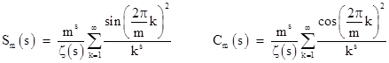
Another interesting family of series involves the squares of the trigonometric functions. We define the series

Obviously S₁(s) = 0 and C₁(s) = 1, and for all m we have S_m(s) + C_m(s) = m^s. For m > 1 we have

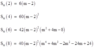
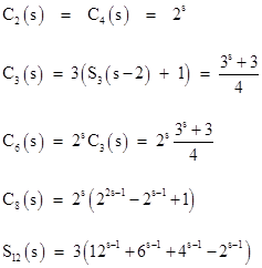
There are some interesting patterns in these values. For example, we have

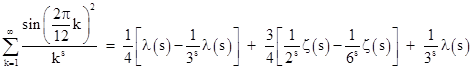
To prove the expression for S₁₂(s), we note that the numerators sin(2πk/12)² have the values 1/4, 3/4, 1, 3/4, 1/2, 0, 1/4, … and so on, repeating every six terms. Therefore, we have

Multiplying through by 12^s/ζ(s) and recalling that λ(s) = (1 – 2^–s)ζ(s), we get the expression for S₁₂(s) noted above.

Evidently C_m(s) is an integer for all positive integers s only for m = 1, 2, 4, 6, 8, and 12. As can be seen from the formula above, C₃(s) is an integer for even s, and a half-integer for odd s.

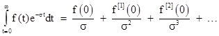
For another approach to the zeta function, recall that the Laplace transform of a function f(t) is given by

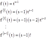
where the superscript f^[k](t) signifies the kth derivative of f(t) with respect to t. If we set f(t) = t^s–1 for some integer s, then we have

and all higher derivatives are zero. Evaluating these at t = 0, we find that

Now, by the geometric series we have

so it follows that

Noting that (s–1)! for any positive integer equals the gamma function Γ(s), we have

which converges for any complex s with real part greater than 1. This was Riemann’s starting point in his famous paper on the number of primes less than a certain value. By complex integration of the “alternating” form of this integral, he found an analytic continuation of this function that converges over the entire complex plane, equivalent to equation (5) above. From this Riemann derived the functional equation, relating the values of ζ(s) and ζ(1–s):

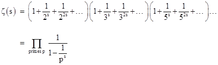
The relevance of the zeta function to the sequence of primes can be seen by noting (as Euler did in 1749) that since every natural number has a unique factorization as a product of primes, ζ(s) can be expressed as

Euler also noted that if there were only a finite number of primes, then the product with (say) s = 1 would have a finite value, but we know (as proven above) that the harmonic series (i.e., ζ(1)) diverges. Therefore, the number of primes must be infinite.

There are some interesting physical applications of the analytically continued zeta function. For example, quantum field theory predicts the existence of a small force between parallel conducting plates. This is called the Casimir effect, attributed to the change in the available energy modes for the quantum vacuum as a function of the distance between the plates. The energy of each standing wave mode is proportional to the frequency, which is inversely proportional to the wavelength. Letting L denote the distance between the plates, and considering only a single dimension, the possible wavelengths for standing waves between the plates are L, L/2, L/3, …, so the energy contributions are proportional to 1, 2, 3, …  (A similar analysis of the spectrum of blackbody radiation based on the equi-partition theorem led the “ultra-violet catastrophe” and hence to Planck’s discovery of quantum theory.) Therefore, the total energy of the vacuum fluctuations between the plates is, according to this reasoning, proportional to the infinite sum 1 + 2 + 3 + …, which of course diverges. However, replacing that infinite sum with ζ(–1) = –1/12 leads to a prediction that agrees with experimental measurements of the Casimir force, so this is sometimes presented as “proof” that the sum 1 + 2 + 3 + … actually does equal –1/12 in some mysterious physical sense. I think the truth is less mysterious, but still interesting. The force between the plates actually depends on the total energy, not just between the plates but also outside the plates. Quantum field theory predicts infinite values for both of those, but the observable force depends only on how the sum of those two varies with the distance between the plates, which may be just a finite amount if there are complementary changes in the interior and exterior energies. Thus it’s misleading to say the relevant energy is just the (formally infinite) energy between the plates. In addition, it’s implausible that all the infinitely-many frequency modes are physically relevant. There is surely a cutoff frequency (and energy) above which we would not expect standing waves contained between the plates to be physically realistic.

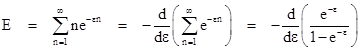
To analyze this, we try to split the inert infinite part of the sum from the relevant “active” part, making use of the concept of a cutoff frequency. Instead of taking the sum of the integers n = 1, 2, 3, …, we will consider the sum of the quantities ne^–εn where ε is a very small constant. If ε = 0 we get the sum of the natural numbers, but for any non-zero value of ε the exponential factor suppresses the frequencies (and hence the energy contributions) above some level. Then we say the energy between the plates is proportional to

Expanding the quantity in parentheses into a series and differentiating term by term, we get

As ε approaches zero the term 1/ε² goes to infinity, as we would expect, but it can be shown that the sum of this infinite term and the corresponding term for the region outside the plates does not depend on the distance between the plates, so those terms don’t contribute to the force. The only contribution to the force is due to the –1/12 term in the expression for the energy between the plates, which is not counter-balanced by any term outside the plates. Thus, the experimentally confirmed Casimir force is not really proportional to the infinite sum 1 + 2 + 3 + …, it is simply proportional to –1/12.

Return to MathPages Main Menu