Eccentrics, Deferents, Epicycles, and Equants

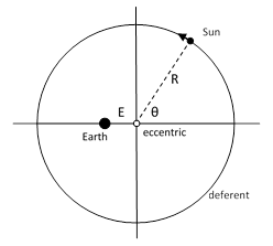
The earliest astronomers imagined the distant stars to be embedded in a crystal sphere, centered on the (presumed stationary) earth, and rotating uniformly. This is consistent with the apparent fact that the stars all move in unison and have constant brightness. The sun, moon, and planets, however, do not move in unison, nor are their individual apparent motions uniform. In addition, the brightnesses of the planets vary, which suggests that their distances from the earth are not constant. The ancients sought to represent the paths of these objects as circles, but even for the relatively simple annual motion of the sun they found it necessary to assume that the circular path was centered on a point – called the eccentric – some distance away from the earth. The circular path itself was called the deferent. This is depicted in the figure below.

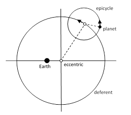
With a suitably chosen radius R, orbital speed, and eccentric (which Hipparchus estimated to be about 1/24 of the radius), this model gave a rough representation of the sun’s motion as seen from the (assumed stationary) earth, but no such model is adequate to account for the irregularities in the motions of the planets. A planet’s rate of progress, as viewed from the earth, varies significantly with time, and each planet actually undergoes temporary periods of retrograde motion (seeming to move backwards). This type of motion obviously can’t be represented by uniform motion in a circle, even if the circle is eccentric. Nevertheless, perhaps because of their attachment to the elementary constructions of Euclidean geometry, or mystical ideas about circles representing perfection, the Greeks were determined to conceive of the planets motions as being circular. Around 150 BC the Greek astronomer Hipparchus developed a model to account for these irregularities while still (arguably) using nothing but uniform circular motion – provided we allow for the composition of such motions. He proposed that each planet moves at uniform speed around a circle – called the epicycle – whose center moves at uniform speed around the deferent, as illustrated below.

This model remained in use for nearly three centuries, and it was still the most widely accepted theory of planetary motion around 150 AD. At that time the great Alexandrian astronomer, Claudius Ptolemy, found that this model didn’t quite match the latest and best observations in all respects. This prompted him to introduce one additional feature, and the resulting model formed the basis of his treatment of the planetary orbits in the Almagest.

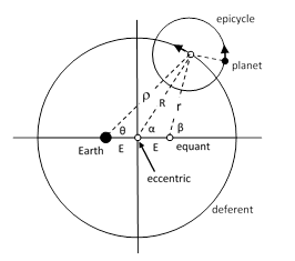
According to Ptolemy’s observations, the center of the epicycle must not move at constant speed around the deferent. It needs to move somewhat faster when it is closer to the earth, and slower when it is further away. It might seem as if he would need to abandon the old preference for uniform circular motion, but he cleverly devised a scheme that allowed him to at least claim that the motion was both circular and uniform – by saying that the path of the center of the epicycle was circular about one point and uniform about another point. The new point was called the equant, which was located on the opposite side of the eccentric, at the same distance as the earth, as shown in the figure below.

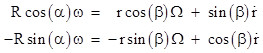
The center of the epicycle moves at a constant distance from the eccentric, but at a constant angular speed about the equant. To determine an explicit expression for angular position of the planet (as a function of time) as seen from the earth, we first need to determine the angular speed of the epicycle center about the eccentric, given that it has a constant angular speed of Ω = dβ/dt about the equant. We can begin with the relations

where R is the constant radius of the deferent and r is the variable distance from the equant to the epicycle center. For future use we note that dividing the first by the second gives

Also, multiplying through the first equation (1) by cos(β) and the second by sin(β), and then subtracting the first result from the second, we get

Taking the differentials of both equations (1) gives

where ω = dα/dt. Multiplying through the first equation by sin(β) and the second by cos(β) and adding the results, we get

Solving this for ω and making use of equation (3) we get

Now, squaring both of the equations (1) and summing the results, we have

The differential of this expression is

Solving this for dr/dt gives

Substituting this expression into equation (5), we get

Solving equation (6) for r and substituting into the above equation, we arrive at the angular speed of the epicycle center about the central point of the deferent

where k = E/R. Integrating this gives the angle of the line from the center of the deferent to the center of the epicycle as an explicit function of time

This represents the angular position of the epicycle’s center as seen from the geometric center of the deferent. To find the corresponding angle θ(t) from the earth to the epicycle center, we begin with the basic relations

Dividing the first by the second, we get

Combining this with equation (2), we see that the tangent of α is the harmonic mean of the tangents of β and θ. In other words, we have

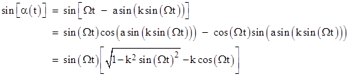
However, this doesn’t lead immediately to an explicit expression for θ in terms of β. To develop such an expression, we make use of equation (8) to express the sine of α(t) as

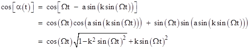
Likewise the cosine of α(t) can be expressed as

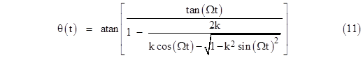
Substituting these expressions into equation (10), simplifying, and solving for θ, we get

Now that we have this expression for θ(t), and the value of α(t) is given by equation (8), we can solve the first equation (9) for the distance r from the earth to the epicycle center at the time t, which gives

Therefore, letting z(t) denote the position of the planet (in complex form) at the time t, and letting w denote the angular speed of the epicycle, we have

Since the angular direction of a complex number doesn’t depend on its magnitude, the direction of the planet (as seen from earth) as a function of time is fully determined in this scheme by specifying the values of Ω, ω, k = E/R, and r/R. Equation (11) is slightly ambiguous because the arctangent is a multi-valued function, and we need to add integer multiples of π to give the pieces of a continuously increasing angular position. However, the ambiguity doesn’t affect (13), because adding π to θ(t) in the first term merely changes the sign of both the numerator and the denominator, leaving the ratio unchanged.

The figure below shows the position of Mars relative to the Earth according to Ptolemy’s model, for a typical ten-year period.

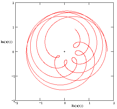
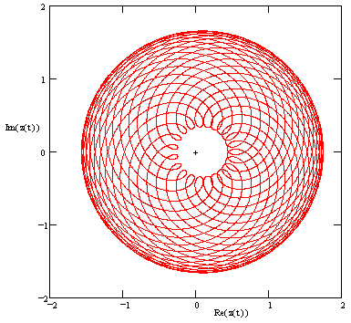
The loops near the points of closest approach to the Earth are the times when Mars appears to be moving backwards (retrograde motion). As can be seen in this figure, the size of the loops differs depending on the direction in the zodiac. If we continue to plot the position of Mars for a period of 100 years, using approximate rational values for the orbital parameters such as eccentricity and rate of rotation, we get a plot such as the one shown below.

This image is slightly misleading, because the rational values selected for the orbital parameters result in a periodic orbit (albeit of very long period), whereas the actual orbital parameters are presumably irrational (unless they are gravitationally synchronized), so the actual orbit of Mars never exactly repeats, and it eventually covers every point within the range. Nevertheless, the figure accurately depicts most features of the orbit. At its point of nearest approach, the distance of Mars from the Earth is about 1/7 of the maximum distance. This agrees with the fact that the minimum and maximum distances between Mars and Earth are about 56 million and 440 million kilometers respectively.

Of course, the absolute distances to the planets were not known during Ptolemy’s time. In fact, even the relative distances were indeterminate in Ptolemy’s scheme, since the pattern of angular positions, and the ratio of apparent brightnesses, for each planet were independent of the scale factor R appearing in equation (13). Hence, although the ratios of the distances of a single planet at different times were represented in Ptolemy’s model, the ratios of the distances to two different planets were not. Some additional information, such as the absolute brightness of each planet, would have been needed in order to determine the ratios of the actual distances of the planets.

Lacking any definite means of ordering the distances, the ancients basically guessed that the planets were ordered according to their overall orbital periods, i.e., the time taken to completely circle the Earth. Hence Saturn was thought to be the most distant (Uranus and Neptune being unknown at the time), then Jupiter, and then Mars. However, the two inner planets behave qualitatively differently, in the sense that they never appear in the opposite direction from the Sun, and their overall orbital periods, as viewed from Earth, are all roughly one year. As a result, there was uncertainty as to the relative distances to these planets, as well as the Sun. The ordering adopted by Ptolemy for the seven wandering objects, from nearest to furthest, was Moon, Mercury, Venus, Sun, Mars, Jupiter, and Saturn. (This ordering was the basis for the naming of our days of the week, as discussed in Saturnday, Sunday, Moonday.)

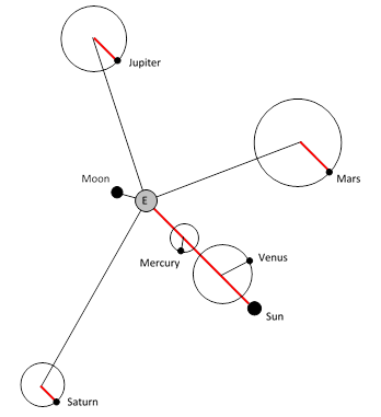
The fact that the equation for each planet’s position contained a logically independent scale factor was a deficiency of Ptolemy’s model. In addition, the model contained what might be regarded as a problem of the opposite kind, namely, that for each of the planet’s (setting aside the Sun and Moon), the value of either Ω or ω was equal to one revolution per year, and moreover the respective phase angles were identical, as depicted schematically in the figure below. (For simplicity we omit the eccentricities.)

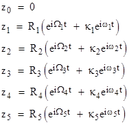
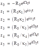
The segments shown in red are always parallel to each other. For the inner planets these are the deferent radii, and for the outer planets these are the epicycle radii. Symbolically, using subscripts 0, 1, 2, .., 5 to denote Earth, Mercury, Venus, …, Saturn respectively, the simple deferent-epicycle model can be expressed in the form

where the R_j scale factors are arbitrary, and the angular velocities are subject to the condition

These equations highlight two unsatisfactory features of Ptolemy’s model. First, the model fails to provide a connection between the individual scale factors. Second, the model does provide an explained connection between some of the angular speeds (not to mention the phases). Thus it is both overly constrained and not constrained enough. It isn’t hard to see that we can use these two “problems” to resolve each other. Suppose we choose the values of the scale factors R_j such that the terms with equal angular speeds all have the same radii. Thus for some value R₀ we require

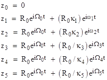
Also, let Ω₀ denote the common angular speed. In these terms we can re-write the planetary equations as

This makes clear the fact that each planet’s motion consists of two parts, one of which is identical for all the planets. If we subtract that term from the positions of all the objects, including the Earth, we get the kinematically equivalent set of relations

This solves both of the “problems” at once, because we now have six independent angular speeds, one for each object (including the Earth), and we have definite relations between the orbital radii, so there is only a single indeterminate scale factor, namely, R₀. Also, the planets are now regarded as moving (to this approximation) uniformly in circular paths, which was the original ideal of the ancient Greeks. This eliminates five epicycles by adding one deferent. In the dedication of “On the Revolutions of Heavenly Spheres”, Copernicus remarked on the unity and coherence of the Sun-centered view:

Having laid down the movements which I attribute to the Earth, I finally discovered by the help of long and numerous observations that if the movements of the other wandering stars are correlated with the circular movement of the Earth, and if the movements are computed in accordance with the revolution of each planet, not only do all their phenomena follow from that, but also this correlation binds together so closely the order and magnitudes of all the planets and of their spheres or orbital circles and the heavens themselves that nothing can be shifted around in any part of them without disrupting the remaining parts and the universe as a whole.

In his 1905 paper on the principle of relativity, Poincare commented on how the transition from the Earth-centered to the Sun-centered model provided an explanation for the appearance of a single constant (the angular speed Ω₀) in the laws governing the behavior of each of the planets. He compared this with the fact, emerging from generalizations of Lorentz’s theorem of corresponding states, that the single constant speed c appears in the laws governing all the fundamental forces of nature. This led Poincare to speculate that, just as in the former case, some new Copernicus might conceive of a new perspective for physics that would account for the apparent coincidence.

Return to MathPages Main Menu