Dirac’s Belt

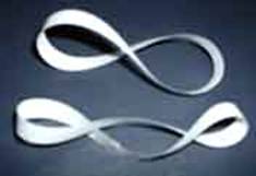
A looped belt possesses both intrinsic and extrinsic structure. If stretching of the surface is not allowed, the local metrical properties are simply those of flat two-dimensional space. Even if stretching is allowed, there are only two distinct intrinsic topologies, namely, the simple two-sided surface with no twist, and the one-sided surface (i.e., a Mobius strip) with a half twist. These two versions are depicted below.

The un-twisted belt is called an orientable surface, because a right-handed figure (for example) remains right-handed, regardless of how it is translated around the manifold. In contrast, the Mobius strip is a non-orientable surface, because a right-handed figure, moved continuously around the loop until arrive back at its starting point, becomes left-handed. An object must be translated around the loop twice in order to be restored to its original position and chirality. In this sense a Mobius strip is reminiscent of spin-1/2 particles in quantum mechanics, since such particles must be rotated through two complete rotations in order to be restored to their original state. After just a single rotation, they are in the negative of their original state, much like the reversed chirality of an object translated just once around a Mobius strip.

The extrinsic structure of a looped belt, as embedded in three-dimensional space, is much complicated than the intrinsic topology, because there are many different ways of arranging and orienting the parts of the loop in space. For example, a loop with one whole twist (or any whole integer numbers of twists) has the same intrinsic topology as an untwisted loop, and yet the embedding of the surface in three-dimensional space is very different. Loops with one and two twists are shown below.

Since the number of twists is a whole integer, the loop can be arranged so that one edge is always “on top”, i.e., nearest the viewer. Hence we can represent such loops by plane figures as shown below.

The twists in these loops may be regarded as extrinsic, because all these loops (with whole integer numbers of twists) share the same intrinsic topology. However, in another sense, the twists can be regarded as intrinsic, because they can’t be removed without cutting the loop.

We can define still another kind of “twist” by stipulating that two or more parts of the loop have fixed spatial positions or orientations. For example, suppose we take the 0-twist loop and move the upper central part downward and the lower central part upward, so they cross over, leading to the diagram shown below.

This resembles the previous “2-twist” diagram, but the “over-under” pattern is different, and it’s easy to see that this diagram still represents a loop with zero twist. In fact there are infinitely many different representations of 0-twist loops, all of which can transformed back to the simple “circular” representation if no additional constraints are imposed. However, if we stipulate that two or more parts of the belt have fixed orientations and spatial positions, we find that some representations of the 0-twist loop cannot be transformed back to the “circle”. For example, suppose we label two points on the 0-twist loop as shown below.

There are two ways of transforming this back to the “circle” form. We could move point A upward and point B downward, or we could axially rotate (i.e., twist) the belt at either of the points A or B through one complete turn. (We could also twist each point through half a turn, leading to an “inside out” circle.) However, if we stipulate that points A and B are fixed in both spatial position and orientation, it is not possible to transform this configuration into a proper circle, even if we allow the other parts of the belt to move off the plane. The term “proper circle” signifies that the same edge of the belt is always facing up (toward the viewed). Of course, we could simply apply half a turn to the outer lobes of the above configuration, leading to a simple circular loop, but this would not be a proper circle, because the outer edges would then be facing downward, whereas the edges at A and B would still be upward.

Now consider the configuration represented by

This too has zero twist. It can be formed from a proper circle by twisting A (or B) axially through two complete turns, or by twisting each of A and B axially through one turn (with the appropriate sense), or, equivalently by holding the orientations and A and B fixed and revolving them through one complete revolution about the central point between them in space. We say that A is twisted through 720 degrees relative to B. Unlike the previous case, this configuration can be transformed back to a proper circle while leaving A and B fixed. To gain a clear understanding of how this occurs, and also to see the limitations on this proposition, it’s helpful to first examine open loops, and the correspondence between twists and loops.

Consider for example a segment of belt extending from A to B, and suppose the B end of the belt is twisted axially through one complete turn in the counter-clockwise direction (when viewed from A). This is shown in the left most figure below. Holding the ends fixed, there are two ways of arranging the belt so that there is no axial twist at any point, provided we introduce a loop. The central figure below shows the belt in proper configuration, i.e., such that the same edge of the belt is always facing upward (out of the page), so the belt is free of axial twist, and it loops to the right and upward as we progress from A to B. Alternatively, we can arrange the belt so that it loops to the left and downward, as shown in the right-most figure below.

Both of the loops are free of local twist at every point, and in both cases if the ends are pulled taut, while keeping the orientations of A and B fixed, the loop disappears, and the belt acquires one whole axial twist. On the other hand, if the loop crossing orders were reversed – so that the ascending loop became a descending loop, and vice versa – we would have loops representing one whole clockwise twist, as shown below.

Again, pulling the looped belts taut eliminates the loops and introduces one whole axial twist, this time in the opposite (clockwise) direction. We could characterize any loop by two unit values, D and E, signifying direction and elevation. If, when progressing from A to B, a loop turns to the left, we say D = +1, whereas if it loops to the right we say D = -1. If the loop goes “upward” (meaning the start of the loop passes below the end of the loop) we say E = +1, and if it goes “downward” we say E = -1. Letting T denote the twist for the corresponding taut belt, we can set T = DE, so T = -1 for counter-clockwise twist, and T = +1 for clockwise twist. The value of T is invariant, regardless of which of the two loop representations we choose, and regardless of whether we proceed from A to B, or from B to A. Given any closed belt with any whole number of twists (possibly zero), we can arrange it in proper configuration with zero local twist at every point, and with a finite number of individual loops like the ones shown above. The sum of the T values for the loops as we proceed around the closed belt is invariant (without cutting the loop), and characterizes the number of twists. Hence, even though all such belts have the same intrinsic topology of an orientable surface, they are distinguished by their different twist numbers.

Notice that passing the belt through itself, or, equivalently, looping the belt around one end, takes it from a whole counter-clockwise twist to a whole clockwise twist, meaning that it represents a twist of two whole turns. Conversely, if we take a flat belt and apply two axial rotations to one of the ends (relative to the other), these twists can be removed (while holding the orientations of the ends fixed) simply by looping the belt around one of the ends (in the correct direction). In this sense, we can say that a configuration with two axial twists is “equivalent” to a configuration with no twists at all, because these configurations can be transformed into each other simply by looping the belt around one of the ends. Needless to say, a single twist cannot be transformed away, because the operation of looping the belt around one end is equivalent to applying two twists, so we cannot eliminate an odd number of twists by this operation. This is sometimes regarded as an illustration of a “spin-1/2” object (as in “Dirac’s belt”), because the object doesn’t transform to itself under one whole rotation, but it does transform to itself under two whole rotations.

However, basing the illustration on an open segment of belt isn’t entirely satisfactory, because it doesn’t fully describe the situation. The two ends A and B are depicted as open, but there must be some connection between them to maintain their relative positions and orientations. Whatever this connection may be, we might expect it to interfere with looping the belt around an end. For example, if we hold one end of the belt in our hand, and we wish to loop the middle part of the belt around the end, we ordinarily find it necessary to let go of the end at some point, and reach around the other side of the belt to grasp the end from the other side. This operation is essentially equivalent to cutting the belt and reconnecting it, so the physical “equivalence” of configurations related by this operation is not self-evident. The question is whether it is absolutely necessary to “let go” of the end of the belt in order to eliminate the double twist.

To examine this question, consider a belt with both ends rigidly attached to some base, making it impossible to loop the belt around either end. Such an arrangement is illustrated below.

If we apply two axial twists to the middle of the belt (by rotating the attached disk twice about its axis), and then hold that portion of the belt fixed, can we remove the twist from the belt? Since both ends of the belt are attached to the base, we can’t simplistically loop the belt around the end, as we did in the previous example. Incidentally, we could regard one half of this belt as the “support”, in place of our hand and arm. Notice that both halves of the belt undergo two twists, so if one of those halves is regarded as our arm, we must imagine twisting our arm twice. It turns out that we can indeed remove the two twists without moving the central portion of the belt, because each half of the belt can be looped around the central disk, and can avoid interfering with each other.

By attaching the two ends to the base, we are essentially constructing a closed belt, so we can dispense with base and simply focus on transformations of a closed belt. We know the belt has zero total twist T (as defined above), because we begin with an untwisted closed belt, and we are not cutting the belt at any time. We can fix a particular point on the loop, apply an axial twist to some other point of the loop, and then ask whether that twist can be removed without changing the orientation or position of those two points. We find that a single whole twist cannot be transformed away, but two whole twists can be transformed away. This is such an interesting phenomenon that, even though it’s very well known, it’s worthwhile to examine it from many different points of view, to understand it better. In the twist-free loop domain, the transformation between the simple closed loop (with two fixed points) and the twice-twisted loop is illustrated in the sequence of schematics below.

The transition from (a) to (b) is accomplished by simply sliding the middle portions in opposite directions, with the right-hand sliding over the left. The transition from (b) to (c) is performed by sliding the upper fixed point downward, pulling the upper part of the top lobe down beneath the middle lobe. Of course, this point is supposed to be fixed, but we could accomplish the same transition by stretching the lower portions upwards while keeping the upper point fixed. We’ve allowed the upper point to move slightly just for convenience in drawing. At this stage we note that the branch labeled a lies completely beneath the link crossing over to the b branch. Hence we can make the transition from (c) to (d) by simply pulling in the a branch and placing it over the crossing link. Once this has been done, the branch labeled b lies completely beneath the link crossing over to the a branch, so we can pull that branch inwards and then place it on top of the crossing link, resulting in configuration (e). To go from (e) to (f) we simply slide the upper fixed point upwards, and then we can make the transition to configuration (g) by pulling the central portions of the loop back to their respective original positions.

Configuration (g)  reveals that the links from the lower to the upper fixed point each have two twists. To make this more explicit, we can convert to standard form. Notice that the left side of (g) is of the form

To clarify this, we make the inner node larger and the outer smaller, as shown below. We can move the smaller node freely along the perimeter of the larger, until it passes completely outside the larger node, resulting in two separate loops.

To make the result even more uniform, we can replace the smaller loop with its equivalent, so instead of looping upward to the left (D = H = 1), it loops downward to the right (D = H = -1). Applying the same transformation to both sides of configuration (g), we get

The figure on the left shows explicitly, in the loop domain, that the upper fixed point is twisted twice relative to the lower fixed point. Also, if we begin at the upper fixed point and follow the loop clockwise, we encounter loops the T = -1, -1, +1, and +1, for a total twist of zero, which is to be expected, since we haven’t cut the belt at any stage, so the total twist is the same as for the original circular form. The figure on the right is the equivalent closed belt representation in the twist domain.

Thus we’ve shown that if we define equivalence classes for representations based on whether or not they can be transformed into each other while leaving two labeled points A and B fixed, then we can say that applying a single twist to A relative to B results in a non-equivalent configuration, but applying a double twist places us back in the original configuration class. This symmetry under a 720 degree rotation, but not under a 360 degree rotation, is similar to what is observed for entities being translated around in the manifold of a Mobius strip and, as noted previously, this makes it similar to the behavior of spin-1/2 particles. In a manner of speaking, we can regard one fixed point (say, B) as the environment, and the other (A) as an entity such as a “particle”. The twisting operations can then be regarded as rotations relative to the environment. The belt represents the entanglement between the particle and the surrounding environment, but it also represents the “arms” that establish the spatial relations between the entity and the environment. Dirac was evidently the first to use a belt loop to illustrate the behavior of spin-1/2 particles in quantum mechanics.

Another way of depicting this is as a ball enclosed within a sphere, and connected by means of a belt, as shown in the figure below. Each edge of the belt can also be regarded as a one-dimensional thread, and twist in the belt corresponds to entanglement between the threads. The reasoning with the belt proves that any pair of threads connecting the sphere and the enclosed ball can be un-entangled after two or any even number of complete rotations of the ball about any fixed axis, but not after just one or any odd number of rotations.

Rotating the ball “A” about the vertical axis (while keeping the surrounding sphere fixed) has the effect of twisting the belt. Two whole twists can be “undone” by looping the belts as shown in the right hand figure and then passing the ball through those loops, or, alternatively, holding the ball fixed and pushing the loops around it. This is equivalent to the transformation described previously.

Of course, since the “point” B in this representation wraps around and is connected to both ends of the belt, this situation is essentially identical to a closed loop belt with two labeled points (assuming we allow movement outside the plane). However, this representation tends to obscure the fact that A and B can be seen as equivalent points on a looped belt, and it particularly diverts attention from the fact that the “double rotation” of A relative to B can also be seen as a single revolution of A and B around their mid-point, holding their orientations constant. The latter point of view allows us to see that the so-called “spin-1/2” symmetry under two spatial rotations is really (in some sense) just an ordinary symmetry under one spatial revolution, making it less counter-intuitive. The “sphere and ball” picture makes it nearly impossible to imagine revolving the particle around the environment, even though this is effectively what we are doing when we rotate the ball through two complete turns while holding the sphere motionless. Of course, in this same way we can eliminate a single twist by moving (with fixed orientations) A and B through half a revolution around their mid-point, but leaves the positions of A and B reversed, and also turns the belt inside-out.

Although we say the configuration is “equivalent” under two full rotations of the ball relative to the sphere, because two such configurations can be transformed into each other as described previously, it’s clear that for an actual physical implementation of this arrangement the transformation might not be possible. For example, if the belt is not stretchable and does not have enough slack to complete the intermediate steps, the transformation is not possible. Even if the belt is sufficiently stretchable, there may be an inherent energy barrier, corresponding to the energy required to stretch the belt sufficiently to perform the transformation between two theoretically “equivalent” configurations. In view of this, we might challenge whether it is physically meaningful to regard such configurations as equivalent. There is, however, one context in which it could be argued that the equivalence is exact. Following something like the “sum over all paths” approach to quantum field theory, we can imagine that, given any fixed configuration of the entity and the environment, a superposition of all possible “equivalent” entanglements exists. On this basis, rotating the entity through 720 degrees would literally return it to the identical state (whereas rotating through 360 degrees would not). Of course, this approach implies a superposition of infinitely many “belts” with progressively more and more twists, so we might expect an “ultra-violet catastrophe”, i.e., infinite energy density at the high-frequency end. This might be mitigated by some kind of weighting scheme.

The use of superpositions to achieve actual equivalence between two configurations of a system is appealing because it evades the troublesome question of whether it is legitimate to regard two configurations as “equivalent” simply because they can be transformed into each other by means of a set of qualifying operations. This kind of equivalence tends to conflict with basic informational (i.e., computational) principles. For example, two different configurations of a “Rubik’s cube” may be considered equivalent if there exists a sequence of allowed transformations from one to the other, and yet this transformation may be extremely non-trivial. This concept of equivalence ignores the real differences in complexity of the transformations. For another example, we might assert that an integer N is “equivalent” to its prime factorization F(N), since each of them uniquely determines the other, and yet the transformation from N to F(N) is believed to be irreducibly difficult, requiring exponential computational effort. Granted, the sequence of operations involved in un-twisting Dirac’s belt is trivial in comparison, but in principle the complete neglect of the complexity of “equivalence transformations” seems questionable.

Several other interesting physical phenomena seem to have analogies in the behavior of looped belts, which are distinct from simple “knots” due to the extra structure represented by the surface (orientable or not) of the belt. We have focused on just orientable belts in this note, in fact, on belts with zero overall twist, but non-orientable belts with half-integer twists, and orientable belts with non-zero whole integer twists are also very interesting, and can be placed in rough correspondence with physical particles possessing various whole or half-integer spins. The duality (or complementarity) between the loop and twist domains is also loosely suggestive of conjuugate variables, such as the position and momentum operators, in quantum mechanics.

Another interesting topic is the duality between the twist and loop domains, and how various equivalence classes arise from two different operations (e.g., twisting, and looping a belt around its end) that induce different numbers of net twist. Since looping a belt around its end induces two twists, we have a ratio of two to one, leading to the analogy with spin-1/2 particles, but in the opposite sense this could also be taken as analogous to a spin-2 particle. In general, if two operations induce m and n twists respectively, then we might regard them as representing, in different senses, spin m/n as well as spin n/m. Thus every spin-1/2 particle would have a dual spin-2 particle. Of course, the particles of spin 1 would be their own duals, much as a massless boson like such as a photon can be regarded as its own anti-particle.

On perhaps a more mundane level, the ability of loops to pass through each other is reminiscent of the smoke ring vortex demonstrations of Peter Guthrie Tait, showing how one smoke ring can overtake and “pass through” another, with both emerging intact after they separate. On the level of elementary particles, it’s interesting to think of a particle and its anti-particle as two opposite loops in a belt, and when they come together they cancel out, leaving no loops or twist at all. Conversely, two opposite loops can appear in a previously “empty” belt, analogous to the appearance of particle and anti-particle pairs in quantum field theory. This would be consistent with the notion that the belt actually consists of a superposition of all possible configurations of a belt that are consistent with the given physical arrangement.

It’s also interesting to note how the ends of an open belt can be rotated continuously in space, and yet the belt can be closed in one of only two possible topological forms, homeomorphic to either a cylinder or a Mobius strip. This is reminiscent of how the state vector of a particle has a continuous degree of freedom for spin, and yet when a measurement is performed (i.e., when its isolation is broken) it can be in one of only two possible states, namely, spin up or spin down. It’s also intriguing that this choice is resolved only when closure of the loop occurs. Prior to closure, there is no matter of fact about the correlation between the two ends, even though those ends might have been correlated with the ends of other belts. Only when the ends of a certain belt are brought together and attached to form a closed belt can we say whether the ends are aligned or anti-aligned. This provides an intriguing model of quantum entanglement as demonstrated in EPR experiments. Of course, it remains to explain how the two sets of correlations involving the separate ends of a belt can all be resolved consistently in such a way that the quantum mechanical correlations are maintained when the two ends are brought together. The difficulty is due to the fact that “spin up” and “spin down” are not purely abstract concepts, but actually refer to spatial directions (as in the deflection of paths in a Stern-Gerlach apparatus), and this severely limits the degrees of freedom for the separate sets of distance correlations, which must somehow be mutually consistent when brought together. This is another form of the basic measurement problem in quantum mechanics, which arises from the (apparent) fact that an isolated state vector may be resolved to an eigenvector relative to one environment, while still being in an unresolved superposition relative to another (higher-level) environment.

Return to MathPages Main Menu