Propagation of Pressure and Waves

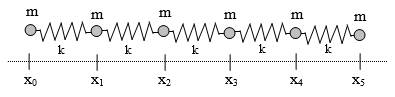
Consider a linear sequence of N point-like particles, each of mass m, connected by springs with spring constants k as illustrated below for N = 5.

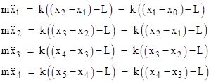
The position of the jth particle at any given time t is x_j(t). The equilibrium length of each spring is L, and the particles are all initially at rest at the locations x_j(0) = jL. We will take as a boundary condition that x₅ is rigidly held in its position, so x₅(t) = 5L for all t. Also, the left-most mass will be driven so that x₀(t) = vt beginning at the time t = 0. The equations of motion for the remaining four particles are

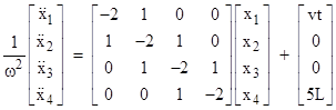
Letting ω² denote the ratio k/m, and re-arranging terms, the equations can be expressed in matrix form as

The parameter ω (equal to the square root of k/m) has units of rad/sec, and represents the characteristic rate of phase change for this system. It’s easy to see that this system of linear differential equations has the particular solution X(t) = P(t) where P is the column vector with components

so we just need to solve the homogeneous system to arrive at the complete solution. Letting M denote the coefficient matrix, the homogeneous system can be written symbolically as

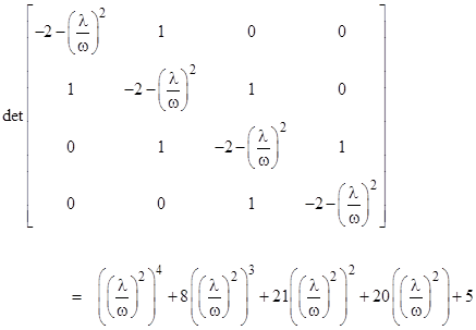
so the eigenvalues can be expressed symbolically as ±ωM^1/2. However, determining the square root of a matrix is not trivial. A more practical approach is to solve for the squares of the eigenvalues of the original matrix equation. The trial solution x_j(t) = A_je^λt , where A_j has units of length and λ has units of time^–1, leads to the characteristic equation

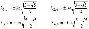
The quartic in (λ/ω)² factors into two quadratics, which can be solved to give the eight purely imaginary eigenvalues of the system

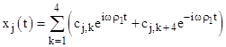
Letting ρ_j denote λ_j/(iω), we can take advantage of the fact that the eigenvalues come in conjugate imaginary pairs to express the solution of the homogeneous equation in the form

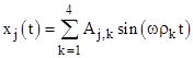
where the coefficients c_j,k are complex constants. This can be expressed as a sum of real-valued sine and cosine functions of real arguments, but we find that the coefficients of the cosine terms must all vanish (to satisfy the conditions of the problem), so we are left with an expression of the form

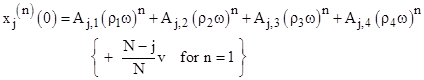
So, combining the homogeneous solution with the particular solution, we know that each of the mass particle positions is of the form

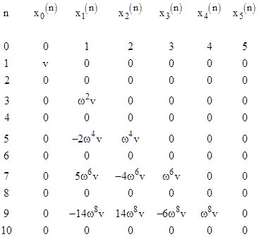
where the coefficients A_j,k are to be determined by the initial conditions. (The cosine terms are all zero.) Making use of the sequence of differentiated system equations

and letting x_j⁽ⁿ⁾ denote the nth derivative of x_j(t) at t = 0, we can construct the following table of initial conditions.

Our general solution automatically satisfies the even-ordered derivatives, because we have set all the coefficients of the cosine terms to zero, so we need only equate the odd-ordered derivatives in the table to the corresponding derivatives of the general solution at t = 0

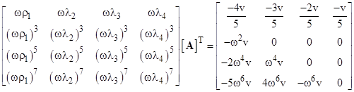
This leads to the system of equations

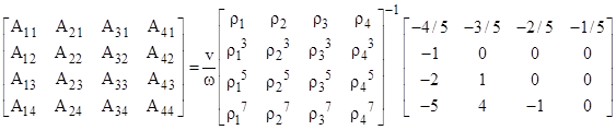
The jth row of the left-hand matrix is a multiple of ω^2j–1, whereas the jth row of the right-hand matrix is a multiple of ω^2j–2. Also, the right hand matrix is a multiple of v. Therefore, if we solve this system by bringing the inverse of the leading matrix over to the right side, we can eliminate all the appearances of v and ω in the matrices, and simply apply a factor of v/ω to the result, so the transpose of the coefficient matrix A is given by

Recall that the values of ρ_j are solutions of

As discussed in Linear Fractional Transformations, polynomials of this type (with coefficients from diagonals of Pascal’s triangle) have the trigonometric solution

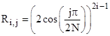
where N = 5 in our example. (We take just one of the square roots of each root ρ² of the (N–1)th degree polynomial.) Thus if we let R denote the matrix whose inverse is taken in the above equation, we can state the components of R explicitly as

Obviously the components of R are dimensionless. The right-most factor in the preceding matrix equation, which we will denote by C, represents the definition of the initial conditions and the particular solution. The elements of the first row are simply –(N–j)/N, and the magnitudes of the elements on the remaining rows can be generated recursively by the relation

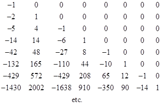
Thus after the first row of we append the first N–2 rows and N–1 columns of the array

The numbers in the first column are obviously the (negative) Catalan numbers, as are the sums of the numbers in each row. Notice that the recurrence relation applies to the first row with the fractional terms as well, and can be exercised in reverse to generate the infinite sequence of previous rows. The components of C are, of course, dimensionless.

In terms of the matrices defined above the positions of the N–1 mass particles as a function of time are given by the row vector

where E(t) is the dimensionless row vector with the components

Recall that P_j(t) = jL + (1–j/N)vt, so if we express the speed v in the form νL where ν is the number of “L-distances” per unit time, and if we note that the homogeneous part of the solution is also a multiple of v, we can divide through by L to give the fully dimensionless equation

where the elements of the first term on the right side are j + (1 – j/N)νt. The coefficient (n/ω) is the ratio of two parameters, each with units of time^-1, but the parameter n signifies a number of L-distances moved by x₀ per unit time, whereas ω represents a number of phase radians per unit time. Multiplying either of these by the length L gives something with units of speed. The quantity Lν equals the speed v of x₀, and the quantity Lω is a characteristic speed related to the phase of the system itself. We will denote this speed by c, and refer to it as the acoustic speed of the system, because it is the speed at which pressure disturbances propagate through the system. To see this, recall that the speed of sound in a material medium is

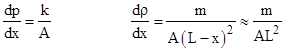
where p is the pressure and ρ is the density. Our mass-spring system is just one-dimensional, but we can arbitrarily assign it a cross-sectional area of A, and we can let x denote a small deviation in the length of a spring from its null-force length L. In these terms, the pressure (force per area) is p = kx/A and the density (mass per volume) is ρ = m/(A(L–x)). From this we have

and therefore

To give an intuitive idea of why Lω should be the phase speed for wave propagation, consider an infinite sequence of mass-springs, and suppose each mass particle is in steady sinusoidal motion, oscillating about its null position, so the particles are always separated by a distance close to the null distance L. The equation of motion for each particle is of the form

Letting ϕ denote the uniform phase shift from one mass to the next, i.e., the phase shift over a distance L, we can put

Substituting into the equation of motion and simplifying, we get

and therefore, since ϕ is small because two adjacent particles will not be far out of phase, we have

Dividing through by ϕ gives Ω/ϕ, which represents the phase change, expressed in units of time^-1, over the distance L from one particle to the next. Therefore, (Ω/ϕ)L = ωL = c is the phase velocity, in agreement with the fluid-mechanical derivation.

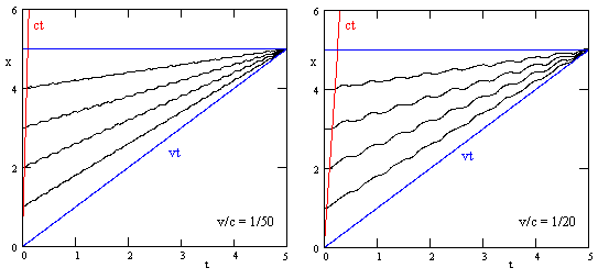
As one would expect, if the speed v of particle x₀ is small compared with c, the result is a quasi-static compression of all the particles, as shown below for the case N = 5 with v/c = 1/50 and v/c = 1/20.

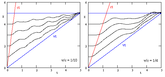
However, as the ratio of v/c increases, we can begin to see the dynamic propagation delay. The figures below are for v/c = 1/10 and v/c = 1/5.

In each case the particles are not appreciably affected until nearly the time when the “ct” line reaches them. In other words, the compression effect propagates at the same speed c as do acoustic waves.

Incidentally, it’s possible for the particles to pass each other dynamically, because the restorative spring force is null for a mutual distance of one unit length, and varies linearly away from that condition. There is nothing singular about the zero-length condition of these idealized springs. A different type of model could be based on, say, mutual inverse-square repulsion, which goes to infinity as the separation goes to zero, so the particles could never pass each other. However, classical force laws of that type do not apply just to neighboring particles but to all the other particles, as instantaneous forces at a distance, so for purposes of illustrating how pressure propagates strictly by “contact forces” it is more convenient to represent the mutual forces as springs (not to mention the fact that the infinite potentials of ideal point-like particles are probably not realistic either).

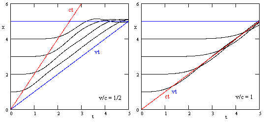
As we increase the ratio of v/c still further, we continue to see that the pressure propagates at essentially the speed c, as shown for the cases v/c = 1/2 and v/c = 1 in the figures below.

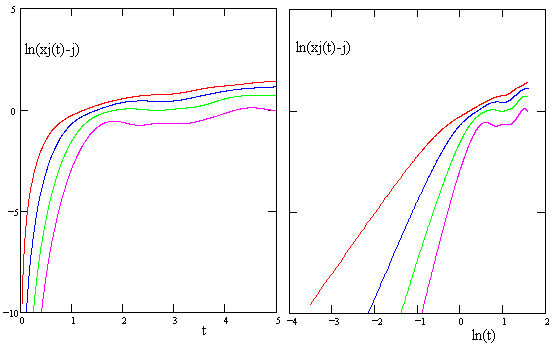
The fact that there is almost no response at the jth mass particle until x_j(0)/c after the particle at x = 0 begins to move might seem counter-intuitive at first, because we know the jth particle begins to move as soon as the (j–1)th particle begins to move, so they should all begin to move at time t = 0. Of course, this supposition relies on our assumption that each spring transmits force instantaneously as a function of the distance between its endpoints. To model a realistic spring we would need to account for the finite acoustic propagation speed of the spring itself, treating each small part of the spring as an element with a certain mass and restorative force. But we have not done this, so there ought to be some instantaneous action at a distance, and indeed if we examine the initial time period closely, by plotting ln(x_j(t) – j) versus t and ln(t) as shown below, we can see that the motion does begin for all the particles at t = 0. (The plots below are for v/c = 1/4.)

These plots also show that the motion of the jth particle is exponentially small until a characteristic time that is proportional to the distance from the source of the disturbance, consistent with the fact that the jth particle is virtually unmoved until x_j(0)/c after the disturbance begins. This is true even though we are modeling each spring as an instantaneous force transmitter.

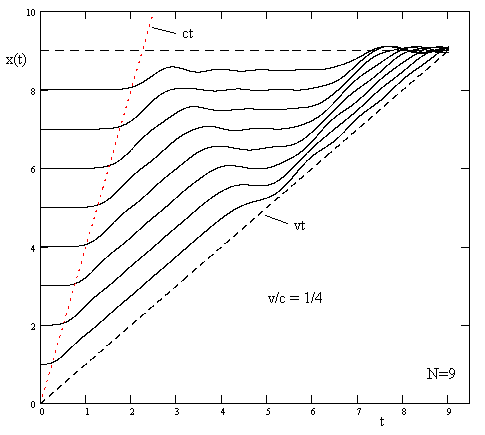
If we increase the number of particles and springs we will gradually approach a truly continuous medium in which the distances over which the forces propagate instantaneously approach zero. For example, the case N = 9 is shown below.

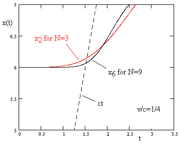
Again we see that the disturbance essentially propagates at the acoustic speed c, but now cutoff at the ct line is even sharper. We can show this by comparing the response of the 6th particle in the N = 9 case with the response of the 2nd particle in the N = 3 case, normalized to the same total distance. This comparison is shown in the figure below.

As expected, the position x₆(t) with N=9 makes a much sharper corner at the acoustic propagation line than does the position x₃(t) with N=3. As we continue to increase N (the number of spring-mass elements into which we divide the overall distance), the corner becomes progressively sharper. In the limit as N goes to infinity - which represents the situation in which all instantaneous force-at-a-distance has been eliminated - the response approaches perfect flatness until reaching the acoustic propagation line.

Thus, despite the fact that there is some non-zero instantaneous response (albeit fantastically small) in the discrete model for any finite N, no matter how large, the acoustic propagation speed becomes an absolute limit as those segments are reduced to zero. One implication is that, if we take the speed of light as an absolute limit on the propagation speed for any energy or information, then the speed limit must apply down to infintessimal scales. On the other hand, the non-zero probability amplitude for a photon to traverse a very small distance at a speed greater than c (according to quantum electro-dynamics) could be interpreted as a propensity for “action at a distance” over those small distances.

Maxwell included some interesting comments on this subject in his Treatise on Electricity and Magnetism. After deriving (in Article 783) the general time-dependent equations for electromagnetic disturbances in terms of the parameters C, K, and m (the specific conductivity, the specific capacity for electrostatic induction, and the magnetic permeability of the medium, respectively), he considers the propagation of such disturbances in two different limiting cases. First, he considers propagation with C=0, i.e., in a non-conducting medium (of which the vacuum would be one example), and shows that the disturbances propagate at the speed

It so happens that the numerical value of this expression equals the speed of light. It was the crowning achievement of Maxwell’s electrodynamic theory that he was able to derive the speed of light in terms of these parameters of electricity and magnetism. Then in Article 801 he considers “the case of a medium in which the conductivity is large in proportion to the inductive capacity. In this case we may leave out the term involving K in the equations of Article 783, and they then become

[and the same for the other components]. Each of these equations is of the same form as the equation of the diffusion of heat given in Fourier’s Traite de la Chaleur.” Maxwell then goes on to discuss the analogy between heat transfer and the diffusion of electromagnetic quantities. For an infinite medium whose initial conditions are known, Fourier had already solved this equation. The value of F at any given point at the time t is the weighted average of the values at every other point, where the weight assigned to a point at a distance r is

Thus at the initial time t = 0 each point just has its own arbitrarily defined value, because the weights for all other point with r greater than 0 are zero. As time increases, the radius r for which there is a significant weight increases – in proportion to the square root of the time. The exponential dependence on time corresponds to the linearity of the logarithmic plots shown above for the motion of the mass particles ahead of the acoustic speed. Then Maxwell makes the interesting remarks

There is no determinate velocity which can be defined as the velocity of diffusion. If we attempt to measure this velocity by ascertaining the time requisite for the production of a given amount of disturbance at a given distance from the origin of disturbance, we find that the smaller the selected value of the disturbance the greater the velocity will appear to be, for however great the distance, and however small the time, the value of the disturbance will differ mathematically from zero. This peculiarity of diffusion distinguishes it from wave-propagation, which takes place with a definite velocity. No disturbance takes place at a given point till the wave reaches that point, and when the wave has passed, the disturbance ceases for ever.

This is reminiscent of how, with our mass-spring “diffusion” system, if we examine the initial portion of x_j(t) more and more closely to determine precisely when it begins to change, we find that it has non-zero change for all t greater than 0, although the magnitude of the change is exponentially small prior to the delay time of D/c. Thus, just as Maxwell says, if we define our threshold small enough, the speed of propagation can be as great as we choose. However, this is only because our model contains implicit action-at-a-distance elements. As noted above, each spring is considered to exert equal and opposite forces at both ends strictly as a function of the difference between the instantaneous positions of the ends. In the limit of a pure contact medium with no extended instantaneous elements, this effect disappears, and the acoustic speed limit becomes absolute for the propagation of any disturbance. It’s odd that Maxwell should have regarded the lack of an absolute speed limit in his artificial “diffusion” example as having physical significance, because he had already shown that the propagation speed for waves was inversely proportional to the square root of K, whereas in the diffusion example he explicity applies the approximation K = 0, i.e., he assumes in this case that the speed of light is infinite, so it should come as no surprise that there is no upper bound on the speed of diffusion under this assumption. Had he worked out the speed of diffusion for non-zero K, he would have found that it does not exceed the speed of wave propagation, as illustrated by the simple mass-spring model.

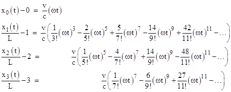
This highlights the profound qualitative difference between the propagation of disturbances in a model with an arbitrarily large (yet finite) number of “distant-action” springs versus the propagation in a continuous model. The former has (in principle) no upper bound on propagation speed, whereas the latter exhibits a strict speed limitation of c for the propagation of any disturbance. The reason for this profound difference involves subtle aspects of mathematical limits, convergence, and existence of functions – the very issues that Fourier is often accused of having overlooked in his treatment of heat flow by means of Fourier series. (Note that as N increases toward infinity, the expression for the position of a particle in the mass-spring system as a sum of sine functions essentially becomes a Fourier series.) We can explain these issues by examining the power series expressions for x_j(t). Recall our table of derivatives of these functions at t = 0. If we consider x_j(t) as a power series in t with constant coefficient, then the nth derivative is n! times the coefficient of tⁿ. Thus we have the following power series for the normalized position functions:

The lowest-degree term of each successive function is two powers of ωt above that of the previous function, which corresponds to the fact that each successive function differs significantly from zero only at progressively larger values of ωt. The “knee” of each curve occurs when ωt exceeds j. Multiplying both quantities by L, replacing ωL with c, and dividing both quantities by c, we find that the normalized position function differs significantly from zero only when t exceeds jL/c.

Nevertheless, each of these functions is, strictly speaking, non-zero for all positive values of t. In other words, for any finite j there is instantaneous action. But what about the limit as N goes to infinity, and not just countable infinity but a continuum? In that case the normalized position function for a particle at the distance D from the origin has no finite-degree term, i.e., it is rigorously zero until the time D/c, so there is no instantaneous action at a distance. This is an example of the “limit paradox”, which is resolved by noting that the limit of a set need not be an element of the set, and need not share all properties of the elements of that set.

Return to MathPages Main Menu