The Laplace Equation and Harmonic Functions

Given a scalar field φ, the Laplace equation in Cartesian coordinates is

This equation arises in many important physical applications, such as potential fields in gravitation and electro-statics, velocity potential fields in fluid dynamics, etc. Typically we are given a set of boundary conditions and we need to solve for the (unique) scalar field φ that is a solution of the Laplace equation and that satisfies those boundary conditions. A solution of Laplace's equation is called a "harmonic function" (for reasons explained below). Since the Laplace equation is linear, the sum of two or more individual solutions is also a solution.

The usual approach to solving the Laplace equation is to seek a "separable" solution given by the product of independent function of x, y, and z, as follows

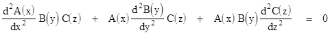
Every solution can be expressed as a sum of (possibly infinitely many) solutions of this form. Inserting this into the Laplace equation and evaluating the derivatives gives

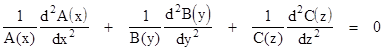
Dividing through by the product A(x)B(y)C(z), this can be written in the form

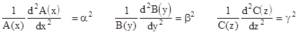
Since x, y, and z can be varied independently, this equation can be identically satisfied only if each of the three terms is a constant, and these three constants sum to zero. It will be convenient to denote these constants by squared quantities, α², β², γ² respectively. Thus we have three separate ordinary differential equations

with the condition α² + β² + γ² = 0. Taking just the first of these, we can re-write it in the form

which the familiar equation of harmonic motion. This is the reason solutions of Laplace's equation are called "harmonic functions". The characteristic polynomial is

whose roots are ±α, so the general solution of the differential equation is

for constants a₁ and a₂. We arrive at similar solutions for B(y) and C(z), so the general solution of the Laplace equation of the form A(x)B(y)C(z) is

where the a_i and b_i are arbitrary constants, and α, β, γ are any complex constants such that α² + β² + γ² = 0. By summing terms of this general form using the techniques of Fourier analysis we can determine the values of these constants necessary to match any given boundary conditions.

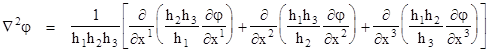
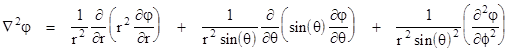
The above analysis is useful when the boundary conditions are easily expressible in terms of Cartesian coordinates, but we often encounter problems that are easier to express in terms of other, possibly curvilinear, coordinate systems. The general form of the Laplacian operator for an arbitrary (differentiable) coordinate system x^k, k = 1,2,3, with the metric tensor g_ij is

where g is the determinant of the covariant metric tensor. If the basis vectors of the coordinate system are mutually orthogonal at each point, the fundamental line element has the diagonal form

where . In this case we have  and g_ij = 0 for all i ¹ j. Also, the non-zero components of the contravariant metric are gⁱⁱ = 1/g_ii , so the Laplacian expressed in terms of orthogonal coordinates has the form

For example, ordinary spherical coordinates r, θ, ϕ where

are orthogonal, i.e., the basis vectors in the r, θ and ϕ directions are mutually orthogonal at each point, so we can express the Laplacian in terms of spherical coordinates by means of the preceding expression. The line element for spherical coordinates is found by simply evaluating the derivatives ds/dr, etc., along the coordinate axes. This gives

and we have h_r = 1, h_θ = r, h_ϕ = rsin(θ). Inserting these into the general expression for the Laplacian in orthogonal coordinates gives

We are often interested in situations with axial symmetry, such as when determining the potential flow around a sphere. In such cases we can take the axis of symmetry over the angle ϕ, so we have ∂φ/∂ϕ = 0, and Laplace's equation reduces to

As in the case of Cartesian rectangular coordinates, we can focus on separable solutions, i.e., solutions of the form φ(r,θ) = A(r)B(θ). Evaluating the Laplacian of this, equating this to zero, and dividing through by A(r)B(θ) gives

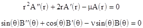
where dots signify derivatives of the function with respect to the argument. Since r and θ are independently variable, this equation can be identically satisfied only if the sum of the first two terms is constant, and the sum of the last two terms is constant. Denoting these constant by μ,ν, we have the two separate ordinary linear differential equations

with the condition μ + ν = 0. We could solve these explicitly, but notice that the first is satisfied by setting A(r) = rⁿ, provided we set μ = n(n+1). Also, if we set B(θ) = cos(θ) the second equation is satisfied with ν = 0. Hence the function φ(r,θ) = rⁿ cos(θ) is a solution of Laplace's equation provided n(n+1) = 0, which implies either n = 0 or n = –1.

More generally, we can consider solutions that are linear combinations of functions of the form

where P_n(x) is a polynomial. Inserting this into the axially symmetric form of Laplace's equation gives

where dotted functions signify derivatives of P_n(x) with respect to x. Dividing through by rⁿ, replacing cos(θ) with "x", and noting that sin(θ)² = 1–cos(θ)², this becomes

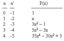
There is a unique (up to a constant factor) polynomial P_n for each value of n(n+1) = k, which implies that each such polynomial is compatible with two distinct values of n, i.e., the two roots n and n' of n² + n = k. Of course, n need not be an integer, but if it is, we can easily determine the polynomial P_n(x) that satisfies the above equation, simply by inserting a polynomial with undetermined coefficients into the equation and solving for the coefficients. The results for the first few values of n are as shown below:

Up to a scale factor, these are the Legendre polynomials (discussed further in the note on Inverse Square Forces and Orthogonal Polynomials). We can express an axially symmetrical solution of the Laplace equation as a linear combination of these individual solutions as follows

where the a_i and b_i are arbitrary constants. The factors of the form P_n(cos(θ)) in this expansion are called zonal harmonics. As an example, the velocity potential of the flow of an ideal, irrotational, frictionless fluid past a stationary sphere of radius R is given by the second zonal harmonic with a₁ = U and b₁ = UR³/2, where U is the free-stream velocity of the fluid moving in the positive x direction (assuming the x axis is our axis of symmetry). Thus we have

The first term is obviously just Ux in Cartesian coordinates, which represents a uniform flow field of constant velocity U in the positive x direction. The second term is a dipole potential, proportional to x/r³. This is the form of the "far field" potential associated with two nearby oppositely charged particles in electrostatics (aligned along the axis of symmetry). It's interesting that the superposition of these two simple fields gives the potential flow field around a sphere, as shown by the fact that the radial velocity vanishes at r = R. (See the note on Potential Flow and d'Alembert's Paradox for more.)

One of the interesting properties of harmonic functions, i.e., continuous functions φ(x,y,z) that satisfy Laplace's equation, is that the mean value of φ on any sphere centered on the point p is equal to the value of φ at the point p. This is called the mean value theorem, and a formal proof of it is presented in Differential Operators and the Divergence Theorem. This theorem is often invoked to prove that a continuous differentiable harmonic function cannot contain a local maximum or minimum, because by definition such points have values of φ properly greater then (resp. less than) the values of φ for all the surrounding points, which would make it impossible for the average on the surface of a sphere surrounding the point to equal the value of φ at that point. In fact, by the same reasoning, if the value of a harmonic function at any given point is increasing in one direction then it must be decreasing in some other direction. (Of course, we don’t actually need the mean value theorem to prove these facts; we can see at a glance that the Laplace equation automatically precludes local maxima and minima, because at any such point all three of the second partial derivatives with respect to x, y, and z would have the same sign, making it impossible for their sum to be zero.)

From this it follows that if the value of a harmonic function φ has the constant value c over an entire surface that completely encloses a region of space, then the value of φ must be c throughout that region. This is because if the value was anything other than c at any point in the interior of the region, then the region must contain a properly highest (or lowest) value, so there must be a point from which the function is decreasing (or increasing) in some directions but not increasing (or decreasing) in any directions, which is impossible.

Having established this, we can also see that the solution of Laplace's equation satisfying a complete set of boundary conditions is unique. To prove this, suppose two distinct harmonic functions φ₁ and φ₂ have the same values on a closed surface, but have different values in the interior of the enclosed region. We know that harmonic functions are additive, so φ₁ – φ₂ is also a harmonic function, and it's value is zero over the closed surface. But this implies the value of this difference is zero throughout the interior region enclosed by the surface (by the preceding proposition), so φ₁ and φ₂ are identical throughout the region.

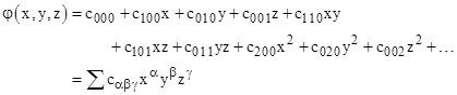
It’s also interesting to consider the mean value theorem in the context of the general power series of a harmonic function. If we expand φ(x,y,z) into a power series about the point p (after shifting the coordinates to place p at the origin), we get an expression of the form

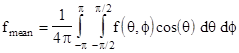
Recall that if θ denotes the “latitude” (zero at the equator) and ϕ the “longitude”, then the mean value of a function f(θ,ϕ) over the surface of a sphere of radius R is given by the double integral

Making the substitutions x = Rcos(ϕ)cos(θ), y = Rsin(ϕ)cos(θ), z = Rsin(θ) into the expression for φ and evaluating the mean value over this sphere gives

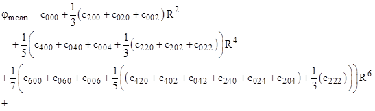
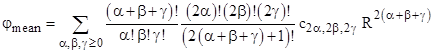
In general we find that only even indices appear, and the mean value can be written as

The constant coefficient in this expression is c₀₀₀, which equals the value of φ at the central point p, corresponding to R = 0. For all other values of R, the mean value theorem asserts that the mean value remains constant, so the coefficients of all non-zero powers of R must vanish. To show that they do, we can substitute the original power series for φ into the Laplace equation and collect terms by powers of x,y,z. We find the coefficient of x^qy^rz^s is

Each of these coefficients must vanish. With q = r = s = 0 this gives

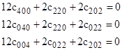
which proves that the coefficient of R² in the series for φ_mean is zero. Likewise for the (q,r,s) combinations (2,0,0), (0,2,0), and (0,0,2) we have the three conditions

Summing these three conditions and dividing by 12 gives

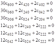
which proves that the coefficient of R⁴ in the double integral for φ_mean is zero. Proceeding on to the next term, with the (q,r,s) combinations (4,0,0), (0,4,0), (0,0,4), (2,2,0), (2,0,2), and (0,2,2) we get the six conditions

Multiplying the first three by 3 and then adding all these expressions together and dividing by 90 gives

which proves that the coefficient of R⁶ in the double integral for φ_mean is zero. This process can be continued indefinitely, corresponding to the fact that the coefficient of each positive power of R is zero, and hence φ_mean = c₀₀₀ for all R.

Return to MathPages Main Menu