Riemannian Geometry

Investigations like the one just made, which begin from general concepts, can serve only to ensure that this work is not hindered by too restricted concepts, and that progress in comprehending the connection of things is not obstructed by traditional prejudices.

                                                                                                       Riemann, 1854

An N-dimensional Riemannian manifold is characterized by a second-order metric tensor g_μν(x) which defines the differential metrical distance along any smooth curve in terms of the differential coordinate components according to

where, as usual, summation is implied over repeated indices in any product. We've written the metric components as g_μν(x) to emphasize that they are not constant, but are allowed to be continuous differentiable functions of position. The fact that the metric components are defined as continuous implies that over a sufficiently small region around any point they may be regarded as constant to the first order. Given any such region in which the metric components are constant we can apply a linear transformation to the coordinates so as to diagonalize the metric, and rescale the coordinates so that the diagonal elements of the metric are all 1 (or –1 in the case of a pseudo-Riemannian metric). Therefore, the metrical relations on the manifold over any sufficiently small region approach arbitrarily close to flatness to the first order in the coordinate differentials. In general, however, the metric components need not be constant to the second order of changes in position. If there exists a coordinate system at a point on the manifold such that the metric components are constant in the first and second order, then the manifold is said to be totally flat at that point (not just asymptotically flat).

Since the metric components are continuous and differentiable, we can expand each component into a Taylor series about any given point p as follows

where g_μν is evaluated at the point p, and in general the symbol g_μν,αβγ... denotes the partial derivatives of g_μν with respect to x^α, x^β, x^γ,... at the point p. Thus we have

and so on. These matrices (which are not necessarily tensors) are obviously symmetric under transpositions of μ and ν, as well as under any permutations of α,β,γ,... (because partial differentiation is commutative). In terms of these symbols we can write the basic line element near the point p as

where the matrices g_μν, g_μν,α, g_μν,αβ, etc., are constants. For incremental paths sufficiently close to the origin, all the terms involving x^α become vanishingly small, and we're left with the familiar formula for the differential line element (ds)² = g_μν dx^μ dx^ν. If all the components of g_μν,α and g_μν,αβ are zero at the point p, then the manifold is totally flat at that point (by definition). However, the converse doesn't follow, because it's possible to define a coordinate system on a flat manifold such that the derivatives of the metric are non-zero at points where the manifold is totally flat. (For example, polar coordinates on a flat plane have this characteristic.)

We seek a criterion for determining whether a given metric at a point p can be transformed into one for which the first and second order coefficients g_μν,α and g_μν,αβ all vanish at that point. By the definition of a Riemannian manifold there exists a coordinate system with respect to which the first partial derivatives of the metric components vanish (local flatness). This can be visualized by imagining an N-dimensional Euclidean space with a Cartesian coordinate system tangent to the manifold at the given point, and projecting the coordinate system (with the origin at the point of tangency) from this Euclidean space onto the manifold in the region near the origin O. With respect to such coordinates the first-order metric components g_μν,α vanish, so the lowest-order non-constant terms of the metric are of the second order, and the line element is given by

In terms of such coordinates the matrix g_μν,αβ contains all the information about the intrinsic curvature (if any) of the manifold at the origin of these coordinates. Naturally the g_μν,αβ coefficients are symmetric in the first two indices because of the symmetry of the metric, and they are also symmetric in the last two indices because partial differentiation is commutative.

Furthermore, we can always transform and rescale the coordinates in such a way that the ratios of the coordinates of any given point P are equal to the ratios of the differential components of the geodesic OP at the origin, and the sum of the squares of the coordinates equals the square of the geodesic distance from the origin. These are called Riemann normal coordinates, since they were introduced by Riemann in his 1854 lecture. (Note that these coordinates are well-defined only out to some finite distance from the origin, beyond which it's possible for geodesics emanating from the origin to intersect with each other, resulting in non-unique coordinates, closely analogous to the accelerating coordinate systems discussed in Section 4.5.) The advantage of these coordinates is that, in addition to ensuring all g_μν,α = 0, they impose two more symmetries on the g_ab,cd, namely, symmetry between the two pairs of indices, and cyclic skew symmetry on the last three indices. In other words, at the origin of Riemann normal coordinates we have

To understand why these symmetries occur, first consider the simple two-dimensional case with x,y coordinates on the surface, and recall that Riemann normal coordinates are defined such that the squared geodesic distance to any point x,y near the origin is given by s² = x² + y². It follows that if we move from the point x,y to the point x+dx, y+dy, and if the increments dx,dy are in the same proportion to each other as x is to y, then the new position is along the same geodesic, and so the squared incremental distance (ds)² equals the sum (dx)² + (dy)². Now, if the surface is flat, this simple expression for (ds)² will hold regardless of the ratio of dx/dy, but for a curved surface it will hold when and only when dx/dy = x/y. In other words, the line element at a point near the origin of Riemann normal coordinates on a curved surface reduces to the Pythagorean line element if and only if the quantity xdy – ydx equals zero. Furthermore, we know that the first-order terms of the metric vanish in Riemann coordinates, so even when xdy – ydx is non-zero, the line element differs from the Pythagorean form only by second-order (and higher) terms in the metric. Therefore, the deviation of the line element from the simple Pythagorean sum of squares must consist of terms of the form x^αx^βdx^μdx^ν, and it must identically vanish if and only if xdy – ydx equals zero. The only expression satisfying these requirements is k(xdy – ydx)² for some constant k, so the line element on a two-dimensional surface with Riemann normal coordinates is of the form

The same reasoning can be applied in N dimensions. If we are given a point (x¹,x²,...,xⁿ) in an N-dimensional manifold near the origin of Riemann coordinates, then the distance (ds)² from that point to the point (x¹+dx¹, x²+dx², ..., x^N+dx^N) is given by the sum of squares of the components if the differentials are in the same proportions to each other as the x^α coordinates, which implies that every expression of the form (x^αdx^β – x^βdx^α) vanishes. If one or more of these N(N–1)/2 expressions does not vanish, then the line element of a curved manifold will contain metric terms of the second order. The most general combination of second-order terms that vanishes if all the differentials are in proportion to the coordinates is a linear combination of the products of two of those terms. In other words, the general line element (up to second order) near the origin of Riemann normal coordinates on a curved surface must be of the form

where the K_μναβ are constants at the given point of the manifold. These coefficients represent the deviation from flatness of the manifold, and they vanish if and only if the curvature is zero (i.e., the manifold is flat). Notice that if all but two of the x and dx are zero, this reduces to the preceding two-dimensional formula involving just the square of (x¹dx² – x²dx¹) and a single curvature coefficient. Also note that in a flat manifold, the quantity x^ρdx^σ – x^σdx^ρ is equal to twice the area of the incremental triangle formed by the origin and the nearby points (x^ρ, x^σ) and (dx^σ,dx^ρ) on the subsurface containing those three points, so it is invariant under coordinate transformations that do not change the scale.

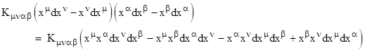
Each individual term in the expansions of the right-hand product in (5) involves four indices (not necessarily distinct). We can expand each product as shown below

Obviously we have the symmetries and anti-symmetries

Furthermore, we see that the value of K for each of the 24 permutations of indices contributes to four of the coefficients in the expanded sum of products, so each of those coefficients is a sum (with appropriate signs) of four K values. Thus the coefficient of x^αx^βdx^μdx^ν is

Both of the identities (3) immediately follow, making use of the symmetries of the K array. It’s also useful to notice that each of the K index permutations is a simple transposition of the indices of the metric coefficient in this expression, so the relationship is invertible up to a constant factor. Using equation (6) we can sum four derivatives of g (with appropriate signs) to give

provided we impose the same skew symmetry on the K values as applies to the g derivatives, i.e.,

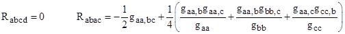
Hence at any point in a differentiable manifold we can define a system of Riemann normal coordinates and in terms of those coordinates the curvature of the manifold is completely characterized by an array R_μναβ = –12K_μναβ . (The factor of -12 is conventional.) We can verify that this is a covariant tensor of rank 4. It is called the Riemann-Christoffel curvature tensor. At the origin of coordinates such that the first derivatives of the metric coefficients vanish, the components of the Riemann tensor are

If we further specialize to a point at the origin of Riemann normal coordinates, we can take advantage of the special symmetry g_ab,cd = g_cd,ab , allowing us to express the curvature tensor in the very simple form

Since the g_μν,αβ are symmetrical under transpositions of [μ,ν] and of [α,β], it's apparent from (8) that if we transpose the first two indices of R_μναβ we simply reverse the sign of the quantity, and likewise for the last two indices. Also, if we swap the first and last pairs of indices we leave the quantity unchanged. Of course, we also have the same skew symmetry on three indices as we have with the K array, i.e., if we hold one index fixed and cyclically permute the other three, the sum of those three quantities vanishes. Symbolically these algebraic symmetries can be summarized as

These symmetries imply that there are only 20 algebraically independent components of the curvature tensor in four dimensions. (See Appendix 7 for a proof.) It should be emphasized that (8) gives the components of the covariant metric tensor only at the origin of a tangent coordinate system (in which the first derivatives of the metric are zero). The unique fully-covariant tensor that reduces to (8) when transformed to tangent coordinates is

where g^μν is the matrix inverse of the zeroth-order metric array g_μν and G_abc is the Christoffel symbol of the first kind as defined in Section 5.4. By inspection of the quantity in brackets we verify that all the symmetry properties of R_abcd continue to apply in this general form, applicable to any curvilinear coordinates. Adding and subtracting g_μν,αβ/2 in this expression, we see that it can be written as

Incidentally, we noted in Section 4.4 that the Riemann tensor can also be interpreted as a representation of the degree to which covariant differentiation in a given metrical manifold does not commute. Appendix 4 explains that the covariant derivative V_α;μ of a vector field V_α is itself a covariant tensor of second order, so we can take the covariant derivative of that to give

It follows that

where R^σ_αμν = g^σκR_καμν. Note that although the Christoffel symbols vanish at the origin of Riemann normal coordinates, their derivatives do not, so it isn’t surprising that covariant differentiation does not commute, even though the first covariant derivative equals the partial derivative at the origin of such coordinates.

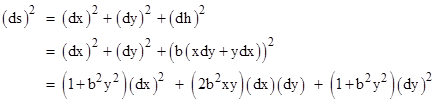
We can illustrate Riemann's approach to curvature with some simple examples in two-dimensional manifolds. First, it's clear that if the geodesic lines emanating from a point on a flat plane are drawn out, and symmetrical x,y coordinates are assigned to every point in accord with the prescription for Riemannian coordinates, we will find that all the components of R_abcd equal zero, and the line element is simply (ds)² = (dx)² + (dy)². Now consider a two-dimensional surface whose height above the xy plane is h = bxy for some constant k. This is a special case of the family of two-dimensional surfaces discussed in Section 5.3. The line element in terms of projected x and y coordinates is

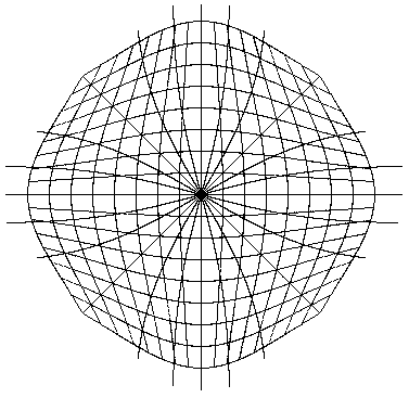
Using the equations of the geodesic paths on this surface given at the end of Section 5.4, we can plot the geodesic paths emanating from the origin, and superimpose the Riemann normal coordinate (X,Y) grid, as shown below.

From the shape of the loci of constant X and constant Y, we infer that the transformation between the original (x,y) coordinates and the Riemann normal coordinates (X,Y) is approximately of the form

Substituting these expressions into the line element and discarding all terms higher than second order (because we are interested only in the region arbitrarily close to the origin) we get

In order for X,Y to be Riemann normal coordinates we must have

and so we must set μ = b²/3. This allows us to write the line element in the form

The last term formally represents four components of the curvature, but the symmetries make them all equal up to sign, i.e., we have

Therefore, we have b² = 12K₁₂₁₂ = –R₁₂₁₂ , which implies that the curvature of this surface at the origin is R₁₂₁₂ = –b², in agreement with what we found in Section 5.3. In general, the Gaussian curvature K, i.e., the product of the two principle curvatures, on a two-dimensional surface, is related to the Riemann tensor by K = R₁₂₁₂ / g where g is the determinant of the metric tensor, which is unity at the origin of Riemann normal coordinates. We also have K = –3k for a surface with the line element (4).

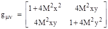
For another example, consider a two dimensional surface whose height above the tangent plane at the origin is h = Ax² + Bxy + Cy². We can rotate the coordinates to bring the height into diagonal form, so we need only consider the form h = Mx² + Ny² for constants M,N, and by re-scaling x and y if necessary we can set N equal to M, so we have a symmetrical paraboloid with height h = M(x² + y²). For x and y coordinates projected onto this surface the metric is

and we have dh = 2M(xdx + ydy). Making this substitution, we find the metric tensor is

At the origin, the first derivatives of the metric all vanish and g = 1, consistent with the fact that x,y is a tangent coordinate system. Also we have the symmetry g_ab,cd = g_cd,ab. Therefore, since g_xy,xy = 4M² and g_xx,yy = 0, we can compute all the components of the Riemann tensor at the origin, such as

which equals the curvature at that point. However, as an alternative, we could make use of the Fibonacci identity

to substitute for (dh)² into the expression for the squared line element. This gives

Rearranging terms, this can be written in the form

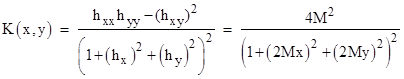
This is not in the form of (4), because the Euclidean part of the metric has a variable coefficient. However, it’s interesting to observe that the ratio of the coefficients of the Riemannian part to the square of the coefficient of the Euclidean part is precisely the Gaussian curvature on the surface

where subscripts on h denote partial derivatives. The numerator and denominator are both determinants of 2x2 matrices, representing different "ground forms" of the surface. This shows that the curvature of a two-dimensional space (or sub-space) at the origin of tangent coordinates at a point is proportional to the coefficient of (xdy–ydx)² in the line element of the surface at that point when decomposed according to the Fibonacci identity.

Returning to general N-dimensional manifolds, for any point p of the manifold we can express the partial derivatives of the metric to first order in terms of these quantities as

The “connection” of this manifold is customarily expressed in the form of Christoffel symbols. To the first order near the origin of our coordinate system the Christoffel symbols of the first kind are

Obviously the Christoffel symbols vanish at the origin of Riemann coordinates, where the first derivatives of the metric coefficients vanish (by definition). We often make use of the first partial derivatives of these symbols with respect to the position coordinates. These can be expressed to the lowest order as

It follows from the symmetries (3) of the partial derivatives of the metric at the origin of Riemann normal coordinates that the first partials of the Christoffel symbols possess the same cyclic skew symmetry, i.e.,

Consequently we have the useful relation (at the origin of Riemann normal coordinates)

Other useful formula can be derived based on the fact that we frequently need to deal with expressions involving the components of the inverse (i.e., contravariant) metric tensor, g^μν(x), which tend to be extremely elaborate expressions except in the case of diagonal matrices. For this reason it's often very advantageous to work with diagonal metrics, noting that every static spacetime metric can be diagonalized. Given a diagonal metric, all the components of the curvature tensor can be inferred from the expressions

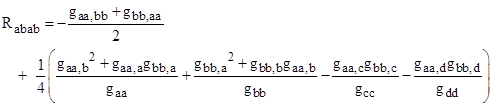
by applying the symmetries of the Riemann tensor. If we further specialize to Riemann coordinates, in terms of which all the first derivatives of the metric vanish, the components of the Riemann curvature tensor for a diagonal metric are summarized by

It is easily verified that this is consistent with the expression for the curvature tensor in Riemann coordinates given in equation (8), together with the symmetries of this tensor, if we set all the non-diagonal metric components to zero.

To find the equations for geodesic paths on a Riemannian manifold, we can take a slightly different approach than we took in Section 5.4. For clarity, we will describe this in terms of a two-dimensional manifold, but it immediately generalizes to any number of dimensions. Since by definition a Riemannian manifold is essentially flat on a sufficiently small scale (a fact which corresponds to the equivalence principle for the spacetime manifold), there necessarily exist coordinates x,y at any given point such that the geodesic paths through that point are simply straight lines. Thus if we let functions x(s) and y(s) denote the parametric equations of the path, where s is the path length, these functions satisfy the differential equation

Any other (possibly curvilinear) system of coordinates X,Y will be related to the x,y coordinates by a transformation of the form

Focusing on just the x expression, we can divide through by ds to give

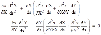
Substituting this into the equation of motion for the x coordinate gives

Expanding the differentiation, we have

Noting the differential identities

we can divide through by ds and then substitute into the preceding equation to give

A similar equation results from the original geodesic equation for y. To abbreviate these expressions we can use superscripts to denote different coordinates, i.e., let

X¹ = X             X² = Y             x¹ = x               x² = y

Then with the usual summation convention we can express both the above equation and the corresponding equation for y in the form

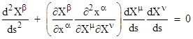
In order to isolate the second derivative of the new coordinates X^α with respect to s, we can multiply through these equations by ∂X^β/∂x^α to give

The partial derivatives represented by ∂X^β/∂x^α are just the components of the transformation from x to X coordinates, whereas the partials represented by  ∂x^α/∂X^μ are the components of the inverse transformation from X to x. Therefore the product of these two is simply the identity transformation, i.e.,

where  signifies the Kronecker delta, defined as 1 if β = μ and 0 otherwise. Hence the first term of (10) is

and so equation (10) can be re-written as

This is the equation for a geodesic with respect to the arbitrary system of curvilinear coordinates X^α. The expression inside the parentheses is the Christoffel symbol G^β_μν, which makes it clear that this symbol describes the relationship between the arbitrary coordinates X^α and the special coordinates x^α with respect to which the geodesics of the surface are unaccelerated. We saw in Section 5.4 how this can be expressed purely in terms of the metric coefficients and their first derivatives with respect to any given set of coordinates. That's obviously a more useful way of expressing them, because we seldom are given special "geodesically aligned" coordinates. In fact, the geodesic paths are essentially what we are trying to determine, given only an arbitrary system of coordinates and the metric coefficients with respect to those coordinates. The formula in Section 5.4 enables us to do this, but it's conceptually useful to understand that

where x essentially represents Cartesian coordinates tangent to the manifold, with respect to which geodesics of the surface (or space) are simple straight lines, and X represents the arbitrary coordinates in terms of which we are trying to express the conditions for geodesic paths. In a sense we can say that the Christoffel symbols describe how our chosen coordinates are curved relative to the geodesic paths at a point. This is why it's possible for the Christoffel symbols to be non-zero even on a flat surface, if we are using curved coordinates (such as polar coordinates) as discussed in Section 5.6.

Return to Table of Contents