5.2  Tensors, Contravariant and Covariant

Ten masts at each make not the altitude

which thou hast perpendicularly fell.

Thy life’s a miracle. Speak yet again.

                                 Shakespeare

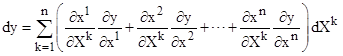
One of the most important relations involving continuous functions of multiple continuous variables (such as coordinates) is the formula for the total differential. In general if we are given a smooth continuous function y = f(x¹,x²,...,xⁿ) of n variables, the incremental change dy in the variable y resulting from incremental changes dx¹, dx², ..., dxⁿ in the variables x¹, x², ... , xⁿ is given by

where ∂y/∂xⁱ is the partial derivative of y with respect to xⁱ. (The superscripts on x are just indices, not exponents.) The scalar quantity dy is called the total differential of y. This formula just expresses the fact that the total incremental change in y equals the sum of the "sensitivities" of y to the independent variables multiplied by the respective incremental changes in those variables. (See Appendix 2 for a slightly more rigorous definition.)

If we define the vectors

then dy equals the scalar (dot) product of these two vectors, i.e., we have dy = g×d. Regarding the variables x¹, x²,..., xⁿ as coordinates on a manifold, the function y = f(x¹,x²,...,xⁿ) defines a scalar field on that manifold, g is the gradient of y (often denoted as ), and d is the differential position of x (often denoted as dx), all evaluated about some nominal point [x¹,x²,...,xⁿ] on the manifold.

The gradient g =  is an example of a covariant tensor, and the differential position d = dx is an example of a contravariant tensor. The difference between these two kinds of tensors is how they transform under a continuous change of coordinates. Suppose we have another system of smooth continuous coordinates X¹, X², ..., Xⁿ defined on the same manifold. Each of these new coordinates can be expressed (in the region around any particular point) as a function of the original coordinates, Xⁱ = Fⁱ(x¹, x², ..., xⁿ), so the total differentials of the new coordinates can be written as

Thus, letting D denote the vector [dX¹,dX²,...,dXⁿ] we see that the components of D are related to the components of d by the equation

This is the prototypical transformation rule for a contravariant tensor of the first order. On the other hand, the gradient vector g =  is a covariant tensor, so it doesn't transform in accord with this rule. To find the correct transformation rule for the gradient (and for covariant tensors in general), note that if the system of functions Fⁱ is invertible (which it is if and only if the determinant of the Jacobian is non-zero), then the original coordinates can be expressed as some functions of these new coordinates, xⁱ = fⁱ(X¹, X², ..., Xⁿ) for i = 1, 2, .., n. This enables us to write the total differentials of the original coordinates as

If we now substitute these expressions for the total coordinate differentials into equation (1) and collect by differentials of the new coordinates, we get

Thus, the components of the gradient of g of y with respect to the Xⁱ coordinates are given by the quantities in parentheses. If we let G denote the gradient of y with respect to these new coordinates, we have

This is the prototypical transformation rule for covariant tensors of the first order. Comparing this with the contravariant rule given by (2), we see that they both define the transformed components as linear combinations of the original components, but in the contravariant case the coefficients are the partials of the new coordinates with respect to the old, whereas in the covariant case the coefficients are the partials of the old coordinates with respect to the new.

The key attribute of a tensor is that it's representations in different coordinate systems depend only on the relative orientations and scales of the coordinate axes at that point, not on the absolute values of the coordinates. This is why the absolute position vector pointing from the origin to a particular object in space is not a tensor, because the components of its representation depend on the absolute values of the coordinates. In contrast, the coordinate differentials transform based solely on local information.

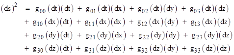
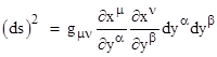
So far we have discussed only first-order tensors, but we can define tensors of any order. One of the most important examples of a second-order tensor is the metric tensor. Recall that the generalized Pythagorean theorem enables us to express the squared differential distance ds along a path on the spacetime manifold to the corresponding differential components dt, dx, dy, dz as a general quadratic function of those differentials as follows

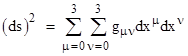
Naturally if we set g₀₀ = −g₁₁ = −g₂₂ = −g₃₃ = 1 and all the other g_ij coefficients to zero, this reduces to the Minkowski metric. However, a different choice of coordinate systems (or a different intrinsic geometry, which will be discussed in subsequent sections) requires the use of the full formula. To simplify the notation, it's customary to use the indexed variables x⁰, x¹, x², x³ in place of t, x, y, z respectively. This allows us to express the above metrical relation in abbreviated form as

To abbreviate the notation even more, we adopt Einstein's convention of omitting the summation symbols altogether, and simply stipulating that summation from 0 to 3 is implied over any index that appears more than once in a given product. With this convention the above expression is written as

Notice that this formula expresses something about the intrinsic metrical relations of the space, but it does so in terms of a specific coordinate system. If we considered the metrical relations at the same point in terms of a different system of coordinates (such as changing from Cartesian to polar coordinates), the coefficients g_μν would be different. Fortunately there is a simple way of converting the g_μν from one system of coordinates to another, based on the fact that they describe a purely localistic relation among differential quantities. Suppose we are given the metrical coefficients g_μν for the coordinates x^α, and we are also given another system of coordinates y^α that are defined in terms of the x^α by some arbitrary continuous functions

Assuming the Jacobian of this transformation isn't zero, we know that it's invertible, and so we can just as well express the original coordinates as continuous functions (at this point) of the new coordinates

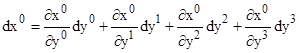
Now we can evaluate the total derivatives of the original coordinates in terms of the new coordinates. For example, dx⁰ can be written as

and similarly for the dx¹, dx², and dx³. The product of any two of these differentials, dx^μ and dx^ν, is of the form

(remembering the summation convention). Substituting these expressions for the products of x differentials in the metric formula (5) gives

The first three factors on the right hand side obviously represent the coefficient of dy^αdy^β in the metric formula with respect to the y coordinates, so we've shown that the array of metric coefficients transforms from the x to the y coordinate system according to the equation

Notice that each component of the new metric array is a linear combination of the old metric components, and the coefficients are the partials of the old coordinates with respect to the new. Arrays that transform in this way are called covariant tensors.

On the other hand, if we define an array A^μν with the components (dx^μ/ds)(dx^ν/ds) where s denotes a path parameter along some particular curve in space, then equation (2) tells us that this array transforms according to the rule

This is very similar to the previous formula, except that the partial derivatives are of the new coordinates with respect to the old. Arrays whose components transform according to this rule are called contra-variant tensors.

When we speak of an array being transformed from one system of coordinates to another, it's clear that the array must have a definite meaning independent of the system of coordinates. We could, for example, have an array of scalar quantities, whose values are the same at a given point, regardless of the coordinate system. However, the components of the array might still be required to change for different systems. For example, suppose the temperature at the point (x,y,z) in a rectangular tank of water is given by the scalar field T(x,y,z), where x,y,z are Cartesian coordinates with origin at the geometric center of the tank. If we change our system of coordinates by moving the origin, say, to one of the corners of the tank, the function T(x,y,z) must change to T(x−x₀, y−y₀, z–z₀). But at a given physical point the value of T is unchanged.

Notice that g₂₀ is the coefficient of (dy)(dt), and g₀₂ is the coefficient of (dt)(dy), so without loss of generality we could combine them into the single term (g₂₀ + g₀₂)(dt)(dy). Thus the individual values of g₂₀ and g₀₂ are arbitrary for a given metrical equation, since all that matters is the sum (g₂₀ + g₀₂). For this reason we're free specify each of those coefficients as half the sum, which results in g₂₀ = g₀₂. The same obviously applies to all the other diagonally symmetric pairs, so for the sake of definiteness and simplicity we can set g_ab = g_ba. It's important to note, however, that this symmetry property doesn't apply to all tensors. In general we have no a priori knowledge of the symmetries (if any) of an arbitrary tensor.

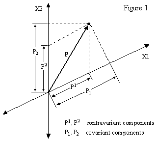
Incidentally, when we refer to a vector (or, more generally, a tensor) as being either contravariant or covariant we're abusing the language slightly, because those terms really just signify two different conventions for interpreting the components of the object with respect to a given coordinate system, whereas the essential attributes of a vector or tensor are independent of the particular coordinate system in which we choose to express it. In general, any given vector or tensor (in a metrical manifold) can be expressed in both contravariant and covariant form with respect to any given coordinate system. For example, consider the vector P shown below.

We should note that when dealing with a vector (or tensor) field on a manifold each element of the field exists entirely at a single point of the manifold, with a direction and a magnitude, as opposed to an arrow extending from one point in the manifold to another. (For example, we might have a vector field describing the direction and speed of the wind at each point in a given volume of air.) However, for the purpose of illustrating the relation between contravariant and covariant components, we are focusing on simple displacement vectors in a flat metrical space, which can be considered to extend from one point to another.

Figure 1 shows an arbitrary coordinate system with the axes X1 and X2, and the contravariant and covariant components of the position vector P with respect to these coordinates. As can be seen, the jth contravariant component consists of the projection of P onto the jth axis parallel to the other axis, whereas the jth covariant component consists of the projection of P into the jth axis perpendicular to that axis. This is the essential distinction (up to scale factors) between the contravariant and covariant ways of expressing a vector or, more generally, a tensor. (It may seem that the naming convention is backwards, because the "contra" components go with the axes, whereas the "co" components go against the axes, but historically these names were given on the basis on the transformation laws that apply to these two different interpretations.)

If the coordinate system is "orthogonal" (meaning that the coordinate axes are mutually perpendicular) then the contravariant and covariant interpretations are identical (up to scale factors). This can be seen by imagining that we make the coordinate axes in Figure 1 perpendicular to each other. Thus when we use orthogonal coordinates we are essentially using both contravariant and covariant coordinates, because in such a context the only difference between them (at any given point) is scale factors. It’s worth noting that "orthogonal" doesn't necessarily imply "rectilinear". For example, polar coordinates are not rectilinear, i.e., the axes are not straight lines, but they are orthogonal, because as we vary the angle we are always moving perpendicular to the local radial axis. Thus the metric of a polar coordinate system is diagonal, just as is the metric of a Cartesian coordinate system, and so the contravariant and covariant forms at any given point differ only by scale factors (although these scale factor may vary as a function of position). Only when we consider systems of coordinates that are not mutually perpendicular do the contravariant and covariant forms differ (at a given point) by more than just scale factors.

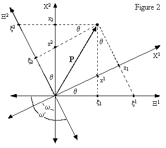
To understand in detail how the representations of vectors in different coordinate systems are related to each other, consider the displacement vector P in a flat 2-dimensional space shown below.

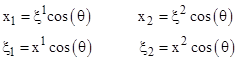
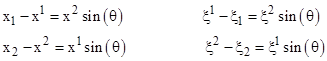
In terms of the X coordinate system the contravariant components of P are (x¹, x²) and the covariant components are (x₁, x₂). We’ve also shown another set of coordinate axes, denoted by Ξ, defined such that Ξ¹ is perpendicular to X², and Ξ² is perpendicular to X¹. In terms of these alternate coordinates the contravariant components of P are (ξ¹, ξ²) and the covariant components are (ξ₁, ξ₂). The symbol ω signifies the angle between the two positive axes X¹, X², and the symbol ω′ denotes the angle between the axes Ξ¹ and Ξ². These angles satisfy the relations ω + ω′ = π and θ = (ω′−ω)/2. We also have

which shows that the covariant components with respect to the X coordinates are the same, up to a scale factor of cos(θ), as the contravariant components with respect to the Ξ coordinates, and vice versa. For this reason the two coordinate systems are called "duals" of each other. Making use of the additional relations

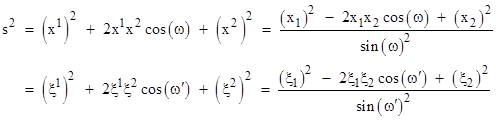
the squared length of P can be expressed in terms of any of these sets of components as follows:

In general the squared length of an arbitrary vector on a (flat) 2-dimensional surface can be given in terms of the contravariant components by an expression of the form

where the coefficients g_uv are the components of the covariant metric tensor. This tensor is always symmetrical, meaning that g_uv = g_vu, so there are really only three independent elements for a two-dimensional manifold. With Einstein's summation convention we can express the preceding equation more succinctly as

From the preceding formulas we can see that the covariant metric tensor for the X coordinate system in Figure 2 is

whereas for the dual coordinate system Ξ the covariant metric tensor is

noting that cos(ω′) = −cos(ω). The determinant g of each of these matrices is sin(ω)², so we can express the relationship between the dual systems of coordinates as

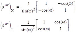
We will find that the inverse of a metric tensor is also very useful, so let's use the superscripted symbol g^uv to denote the inverse of a given g_uv. The inverse metric tensors for the X and Ξ coordinate systems are

Comparing the left-hand matrix with the previous expression for s² in terms of the covariant components, we see that

so the inverse of the covariant metric tensor is indeed the contravariant metric tensor. Now let's consider a vector x whose contravariant components relative to the X axes of Figure 2 are x¹, x², and let’s multiply this by the covariant metric tensor as follows:

Remember that summation is implied over the repeated index u, whereas the index v appears only once (in any given product) so this expression applies for any value of v. Thus the expression represents the two equations

If we carry out this multiplication we find

which agrees with the previously stated relations between the covariant and contravariant components, noting that sin(θ) = cos(ω). If we perform the inverse operation, multiplying these covariant components by the contravariant metric tensor, we recover the original contravariant components, i.e., we have

Hence we can convert from the contravariant to the covariant versions of a given vector simply by multiplying by the covariant metric tensor, and we can convert back simply by multiplying by the inverse of the metric tensor. These operations are called "raising and lowering of indices", because they convert x from a superscripted to a subscripted variable, or vice versa. In this way we can also create mixed tensors, i.e., tensors that are contravariant in some of their indices and covariant in others.

It’s worth noting that, since x_u = g_uv x^u , we have

Many other useful relations can be expressed in this way. For example, the angle θ between two vectors a and b is given by

These techniques immediately generalize to any number of dimensions, and to tensors with any number of indices, including "mixed tensors" as defined above. In addition, we need not restrict ourselves to flat spaces or coordinate systems whose metrics are constant (as in the above examples). Of course, if the metric is variable then we can no longer express finite interval lengths in terms of finite component differences. However, the above distance formulas still apply, provided we express them in differential form, i.e., the incremental distance ds along a path is related to the incremental components dx^j according to

so we need to integrate this over a given path to determine the length of the path. These are exactly the formulas used in 4-dimensional spacetime to determine the spatial and temporal "distances" between events in general relativity.

For any given index we could generalize the idea of contravariance and covariance to include mixtures of these two qualities in a single index. This is not ordinarily done, but it is possible. Recall that the contravariant components are measured parallel to the coordinate axes, and the covariant components are measured normal to all the other axes. These are the two extreme cases, but we could define components with respect to directions that make a fixed angle relative to the coordinate axes and normals. The transformation rule for such representations is more complicated than either (6) or (8), but each component can be resolved into sub-components that are either purely contravariant or purely covariant, so these two extreme cases suffice to express all transformation characteristics of tensors.

Return to Table of Contents