Equidistant Curves

Euclid defined parallel straight lines as “straight lines which, being in the same plane and being produced indefinitely in both directions, do not meet one another in either direction.” Some later authors have been dis-satisfied with this definition, arguing that the negative assertion has no applicability, since it relies on the existence and apprehension of a completed infinity. (Interestingly, analogous concerns have been raised regarding definitions of black holes in general relativity as regions that are not in the causal past of future null infinity.) Several alternative definitions of “parallel” have been proposed, even in ancient times. Among them is the proposal to define parallel lines as lines separated by a constant distant. Parallel straight lines in Euclidean plane geometry do indeed posses this property, provided the “distance” is measured perpendicularly to the lines. However, such a definition relies on the concept of “perpendicular”, which is complementary to “parallel”. Some authors have suggested that, if we are allowed to take perpendicularity for granted, we could give a purely directional definition of parallelism, saying that two curves A and B are (everywhere) parallel if every straight line perpendicular to A is also perpendicular to B. Of course, this again relies on the apprehension of a completed infinity. To avoid this, some authors suggest that we could define parallel straight lines A and B simply by requiring that a single specific straight line perpendicular to A is perpendicular to B, but this is not satisfactory, since we have no guarantee that it would apply to other crossing lines.

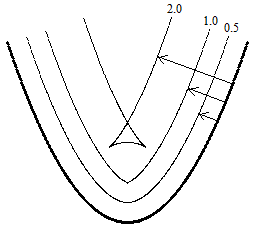
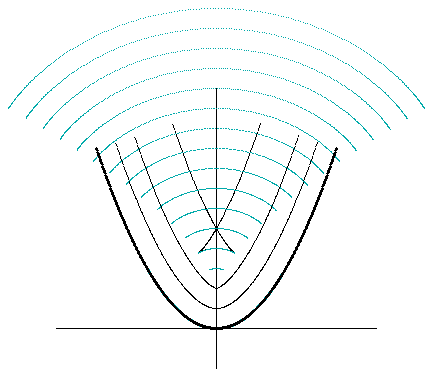
Returning to the “equidistant” definition, we see that it too can only be completely met by apprehending a completed infinity, although in this case it may be said to have some local applicability. Over any finite range of interest we can define a locus of points that are perpendicularly equidistant from a given line, and assert that the locus is parallel to that straight line at least over that range. However, we cannot assert that the locus produced in this way is necessarily a straight line. To see this more clearly, consider the same construction for other kinds of lines, such as circles, parabolas, hyperbolas, etc. In other words, for any plane curve C, consider the locus L of points equidistant from C, where distance is defined perpendicular to C. We will say the locus L is equidistant to C. It happens to be true that any contiguous locus equidistant to a circle is also a circle. (We specify “contiguous” because, strictly speaking, the locus of equidistant points gives two contiguous loci, corresponding to the two different perpendicular directions.) However, the locus of points equidistant to a parabola is not generally a parabola, and may even contain singularities, as shown in the figure below.

For small distances, the interior locus is a smooth curve, though not exactly a parabola, but for larger distances (such as the distance denoted by 2.0 in the above figure) the locus contains singularities and crosses itself, so it is quite different in character from the parabola.

Is equidistance reflexive? In other words, if A is equidistant to B, does it follow that B is equidistant to A? In order for this to be true, each distance segment must be perpendicular to both curves. At first glance, one might think this is not the case, at least for cases when the equidistant locus contains loops, as in the figure above. However, even the interior locus at a distance of 2.0 in that figure actually is perpendicular to the distance segments at every point – except at the two cusp singularities where the slope of the locus is undefined. This is true quite generally. To prove this, suppose the original locus can be expressed (over any given region) in terms of Cartesian coordinates as y = f(x) for some continuous differential function f. Thus we have

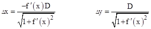
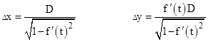
From any given point (x,y) on the original curve C, we need to offset by a vector (Δx, Δy). In order for the offset to be perpendicular to C, and to have the constant length D, the components must satisfy

Therefore we have

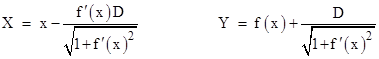
Hence, recalling that y = f(x), the coordinates X,Y of the corresponding point of the locus L are

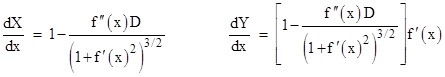
Differentiating these expressions with respect to x, we get

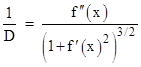
from which it follows that dY/dX = fʹ(x) = dy/dx. Therefore, the slope of the locus L equals the slope of the original curve C at corresponding points, so both curves are perpendicular to the distance segments, and hence equidistantness is reflexive. The only exceptions are when the common factor in dX/dx and dY/dx vanishes, which occurs when

The right hand side is the well-known expression for the curvature of a plane curve, which is the reciprocal of the radius of curvature. Thus the equidistant locus is singular at any location where the radius of curvature of the original curve equals the fixed distance. At such a location, as the distance segment translates along the original curve, it is simply pivoting about a single point of the locus. This proves that equidistantness is reflexive except at singularities, and those are removable in the sense that we can stipulate the appropriate circular arcs at any cusps.

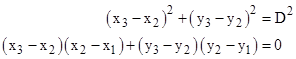
For plotting purposes, it’s useful to note that, given the coordinates of two neighboring points (x₁,y₁) and (x₂,y₂) on the base curve, the coordinates (x_t,y_t) of a point on the equidistant locus must satisfy

Solving the second equation for (y₃−y₂) and substituting into the first, we get

where r is the distance between the two neighboring points on the base curve.

In the case of a parabolic base curve, we can highlight the portion of the equidistant curves (at increasing distances) in between the two singularities, i.e., as x ranges between ±(D^2/3 – 1)^1/2. This gives the emanating arcs as shown below.

The equidistant curves to a hyperbola are somewhat similar, as shown below.

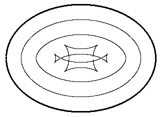
For an ellipse the (inward) tandem curves may have four singularities, as shown in the figure below.

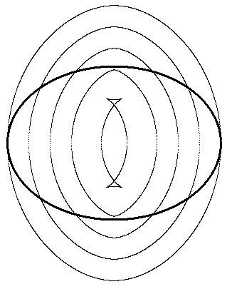
If we continue to increase the “inward” distance, we progress toward an oval shape whose major and minor axes are reversed relative to the base ellipse, as shown in the plot below.

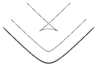
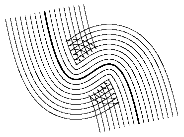
Naturally we can determine the family of equidistant curves for any arbitrary curve, and in general for any local maximum of curvature there arises a “wave” emanating from that region, as illustrated in the figure below, reminiscent of the radiation field versus the near field in wave propagation.

We can also consider perpendicularly equidistant worldlines in spacetime. Consider a worldline C defined by x = f(t) for some continuous differential function f. Thus we have

From any given event (x,t) on the original curve C, we need to offset by a vector (Δx, Δt). In order for the offset to be perpendicular to C (in the Minkowskian sense), and to have the constant Minkowskian length D, the components must satisfy

We can solve these to give

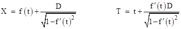
Hence, recalling that x = f(t), the coordinates X,T of the corresponding point of the locus L are

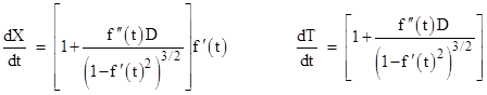
Differentiating these expressions with respect to t, we get

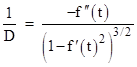
from which it follows that dX/dT = fʹ(t) = dx/dt. Therefore, the slope of the locus L equals the slope of the original curve C at corresponding points, so both curves are perpendicular to the distance segments, and hence equidistantness is reflexive. The only exceptions are when the common factor in dX/dt and dT/dt vanishes, which occurs when

In this expression D represents the distance to the “pivot point” in Born rigid acceleration. Interestingly, the right hand side multiplied by the rest mass of a particle is the longitudinal mass of that particle moving along the worldline C. Recall from the previous note on Born Rigid motion that hyperbolic worldlines are perpendicularly equidistant – in the Minkowskian sense – from other hyperbolic worldlines, with no singularities or cusps. Thus equidistant paths are apparently a more natural concept in Minkowski spacetime than in Euclidean space.

Return to MathPages Main Menu