Quantum Oscillator and Delannoy Numbers

‘Tis thus at the roaring Loom of Time I ply,

And weave for God the Garment thou seest Him by.

                          Carlyle / Goethe

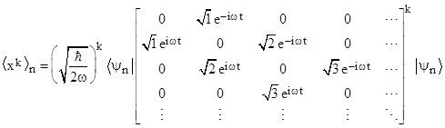
In a note on matrix mechanics we described how the average value (over a cycle of a periodic system with discrete stationary states) of a quantum variable x can be calculated for the nth stationary state by evaluating the expression <x> = <ψ_n|x|ψ_n> where x denotes the matrix corresponding to the variable and ψ_n denotes the eigenvector for the nth stationary state. We also saw how the average value of the square of x can be computed, simply by replacing x and x in that expression with x² and x². In general, the average value of the kth power of x is given by <x^k> = <ψ_n|x^k|ψ_n>. For example, the average value of the kth power of a simple harmonic oscillator in the nth stationary state is

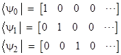
where <ψ_n| and |ψ_n> are the row and column forms (“bra” and “ket”) of the eigenvector corresponding to the nth stationary state. With the diagonalized Hamiltonian having the energy eigenvalues along the diagonal, the row eigenvectors are

and so on, and the corresponding column eigenvectors are the transposes of these. The effect of bracketing a matrix between <ψ_n| and |ψ_n> is to simply select the nth element on the main diagonal of the matrix. Thus the average position coordinate of the simple harmonic oscillator is <x>_n = 0 for all n, because all the elements on the main diagonal of x are zero. Likewise the average value of the squared position coordinate x² for the nth stationary state is the nth diagonal element of x². The square of the x matrix has the values 1, 3, 5, … along the main diagonal, so we have the results

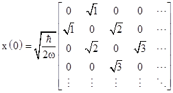
It’s easy to see that <x^k>_n = 0 for all odd integers k, since every odd power of x has zeros on the main diagonal. On the other hand, for even exponents we get non-zero elements on the main diagonal. Notice that the time-dependent phase factors are irrelevant for the values along the diagonal, so we need only consider powers of the matrix

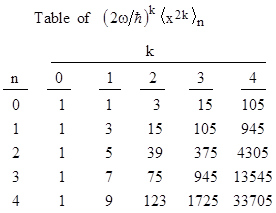
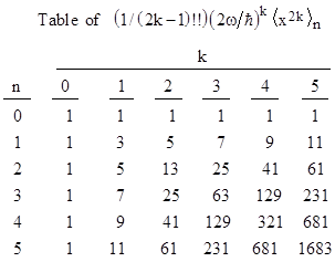
The diagonal terms of the (2k)th powers of this matrix lead to the following table of average values of the (2k)th power of the x coordinate of the nth stationary state of a simple harmonic oscillator.

The values in the top row (n=0) are the “double factorials” given by 1, 1∙3, 1∙3∙5, 1∙3∙5∙7, and so on. If we divide each value of the kth column by the value at the top of that column, we get the table shown below.

These are called the Delannoy numbers, named after the French military officer and amateur mathematician Henri Delannoy (1833-1915). A discussion of these numbers can be found in Theory of Numbers by Edouard Lucas, published in 1891. Clearly in each square of four numbers the lower right hand number is the sum of the other three. For example, 231 = 41 + 61 + 129. This makes it easy to recursively compute the values of the table, and hence the averages of the powers of the position coordinate of a quantum harmonic oscillator.

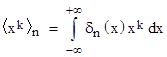
Given a periodic function x(t) we can obviously compute the average values (over one cycle) of x(t)^k for any power k, but the converse is not true, i.e., given the average values of those powers of x we cannot infer the function x(t). We can, however, infer the distribution of x values. There are two different approaches we could take. Perhaps the most direct approach is to let δ_n(x) denote the putative density distribution of x values for the nth stationary state, and then note that the average value of <x^k>_n is given by

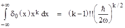
For example, using the average powers for the ground state (n=0) noted above, we can infer that the distribution function δ₀(x) must satisfy the relations

with the understanding that m!! = 0 for even integers m. These relations are satisfied by setting the density function (for unit mass) to

which is just a normal distribution centered on the origin. This is the well-known probability density distribution for the ground state of a simple harmonic oscillator from wave mechanics. The probability density is the square of the wave function u₀(x), so this corresponds to the wave function

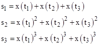
An alternative approach to inferring the individual positions from the averages of the powers of the positions is to attempt to solve for the positions explicitly. Consider first just two values, x(t₁) and x(t₂). Knowing the average of these two values, and also knowing the average of the squares of these two values, we have the quantities

Solving these two equations for the two unknowns x(t₁) and x(t₂), we find that each of those values is a root of the quadratic

where

are the elementary symmetric functions of the roots. Letting x₁ and x₂ denote the roots of the quadratic, we know their values, but the equation is symmetrical so we don’t know which root corresponds to which of the values x(t₁) and x(t₂).

Likewise we could consider the averages of the first, second, and third powers of three values x(t₁), x(t₂), and x(t₃), so we have the three quantities

Solving these three equations for the three unknowns, we find (again) that they are each the roots of a single polynomial, in this case the cubic

where

From this we can compute the values of the three roots x₁, x₂, x₃, but we cannot determine which of these roots corresponds to which of the values x(t₁), x(t₂), and x(t₃). Any permutation of the roots would give the same averages of powers.

Now, for any number N of values of x(t_j), j=1,2,..N, we could in principle carry out this same calculation, determining first the averages of kth powers of those values for k = 1 to N, and then using Waring’s formula to compute the coefficients of the polynomial of degree N whose roots x₁, x₂, …, x_N are those N values of x(t_j). However, since the polynomial is perfectly symmetrical in the roots, we cannot determine which root corresponds to which value of x(t_j). Any permutation of these temporal strands is equivalent in the sense that it gives the same averages of the powers. Letting N increase without limit, we can imagine a nearly continuous sampling of the putative underlying function x(t), and the quantum mechanical equations give us the averages of the kth powers of these samples, from which we can infer the multi-set of values, but only up to permutations. Thus, although we can infer the distribution of the values, such as what percentage of values are in any particular range, we can’t assign any continuous trajectory to the x values. Each stationary state is therefore just characterized by a distribution, rather than a trajectory.

There are some subtle issues here. First, interpreting the distribution of the x values as a probability density relies on the premise that the “samples” are equally probable and cover the cycle uniformly. For example, if we began with an actual trajectory x(t) we would take our samples at equally spaced increments of time (equal phases), since this presumably represents a uniform measure. However, since we have no actual trajectory, we can only assume that the averages given by the quantum mechanical equation are consistent with a valid probabilistic interpretation of the distribution of the roots inferred from those averages. This is consistent with, for example, Whittaker’s statement that

By the correspondence principle we infer that a diagonal element x_nn of the matrix representing a variable x is to be interpreted as the average value of the variable x in the stationary state corresponding to the quantum number n, when all phases are equally probable.

A second subtlety concerns what it actually means to talk about the value of a variable (such as the position coordinate) in a stationary state. It isn’t obvious how this “value” relates to what we would actually measure if we perform a measurement of that variable on the system. To understand the difficulty, consider again the classical oscillator (as discussed in the previous note) with the position coordinate given by

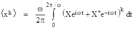
where the constants of integration X and X^* are complex conjugates. This is a simple sinusoidal function with an amplitude of 2|X| and some arbitrary phase angle. The average value of x(t)^k over one cycle is

Just as in the quantum mechanical case, for odd powers the average value is always zero. For even powers we get

For convenience we define y = (x/|X|)², and then we have for any set of equiprobable y values

The normalized x values are the square roots of the y values, so they come in pairs of opposite signs. Thus to determine N values of x we need only determine τ = N/2 values of y. Letting s_j denote the sum of the jth powers of a set of τ equiprobable values of y, we have

Making use of the expression for the first three elementary symmetric σ₁, σ₂, σ₃ given above, along with the expression

we have

With τ = 4 this gives the quartic equation

which has the four roots given by

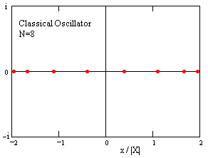
The eight values of the position coordinate x are the positive and negative square roots of these values, namely, ±0.390, ±1.111, ±1.663, and ±1.962. These values are shown in the figure below.

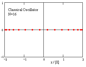
In the same way we can shown that a set of sixteen values of x that have the required sums of kth powers for k = 1 to 16 for a classical harmonic oscillator must be the sixteen values given by

A plot of these sixteen values is shown below.

As we increase N these values approach a continuous locus ranging from -2 to +2 with a density proportional to the fraction of time spent at that position. This represents the probability density for the particle being in any specified range.

Now, one might think the x values for a quantum oscillator inferred from the average values of the powers of x would yield a qualitatively similar result, consisting of a distribution of N real values distributed on a finite range. However, the results are actually significantly different, because the averages of the normalized powers of x for a quantum oscillator in the ground state (n=0) do not equal the central binomial coefficients 1, 2, 6, 20, 70, 252, …, as they do in the classical case, but rather the double-factorials 1, 1, 3, 15, 105, 945, … In other words, instead of (1) we have

In terms of the normalized variable  we have

Again letting s_j denote the sum of the jth powers of a set of τ equiprobable values of y, we now have

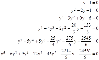
Using the expressions for the elementary symmetric functions for a set of τ values of y, for τ = 1 to 6, we find that these values must be respectively the roots of

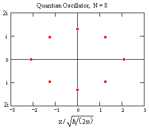
For N=8 we get the multi-set of normalized x values shown in the figure below.

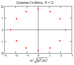
In general, the “values” of x in the ground state that we infer from the requirement to match the quantum mechanical expressions for the averages of the first k powers of x with k samples are complex, so not only are we unable to place them into a definite sequence, we cannot even directly identify these “values” with real measurements. This is consistent with the fact that the particle in a quantum oscillator does not have a definite classical trajectory, nor even a definite classical position and momentum in any given stationary state. For N=12 we get the multi-set of normalized x values shown in the figure below.

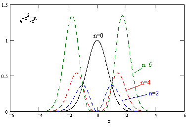
Another significant difference between the classical and quantum result is that as we consider larger values of N the distances of the normalized x values from the origin continue to increase. This is a consequence of the fact that the main contributions to the averages of the higher powers of x come from progressively further away from the origin, as indicated in the figure below.

Of course, this does not imply that the quantum averages cannot be consistent with a distribution of real-valued position coordinates. We saw previously how to infer the density distribution of real-valued positions consistent with all the quantum mechanical averages. Likewise if we allow a sufficiently large number of points, distributed appropriately, we could match the first k quantum averages with purely real-valued positions, but only with many more than k points. We arrive at complex-valued positions using the explicit solution method only because we are imposing the requirement to match the first k averages with just k points. As we’ve seen, this approach yields real-valued positions with the correct distribution for the classical averages, but it yields complex-valued positions for the quantum averages. It would be interesting to know if there is any physical significance to the set of complex positions that formally satisfy all the quantum average conditions. This seems unlikely, because in order to match all of the quantum averages we would need to let N increase to infinity, and the multi-set of positions would recede further and further from the origin.

Return to MathPages Main Menu