Magnetic Dipoles

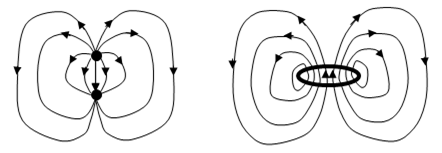
Although electric and magnetic fields, as described by Maxwell’s equations, are formally very similar, there is a striking asymmetry between electricity and magnetism in nature, associated with the apparent non-existence of elementary magnetic charges (i.e., magnetic monopoles) and magnetic current. There do, however, exist what appear to be magnetic dipoles, analogous to electric dipoles consisting of adjacent positive and negative electric charges. It might seem as if the existence of magnetic dipoles is indirect proof of the existence of individual magnetic charges, assuming the only way to produce a dipole field is by juxtaposing two oppositely charged magnetic monopoles. However, there is an alternative way of creating a magnetic “dipole” field without actually using magnetic charges. The alternative is an electric current loop. It can be shown that a circular loop of electric current produces a magnetic field that is (outside a spherical region enclosing the loop) nearly identical to the field of two adjacent and oppositely charged magnetic monopoles (if such things existed). So, we have two possible classical models for the source of “magnetic dipole” fields, one based on the juxtaposition of two oppositely charged magnetic monopoles, and one based on a loop of electric current. These two models, which might be called Coulombic and Amperean dipoles respectively, are illustrated (crudely) below.

Notice that, in the external region away from the charges or current loops, the field lines for the two models point in the same directions, but in the internal regions (in between the charges of the Coulombic dipole, and inside the current loop of the Amperean “dipole”) the field lines point in opposite directions.

It’s often useful to consider these “dipoles” in the limit as the distance between the charges goes to zero, or as the radius of the current loop shrinks to zero, respectively. To maintain a constant dipole “moment”, we require that the charge or current be increased as the size shrinks. In this way we arrive at the idealized concept of a point-like dipole with a given magnetic moment. In the limit, the two models give identical dipole fields (except at the central point itself), so one might think these two models are indistinguishable. However, an important contribution to the behavior of these dipoles comes from the “interior” fields, i.e., the fields in between the poles and inside the loop, where, as we’ve seen, the field lines are actually in the opposite directions in the two models. These contributions remain finite and distinct even in the limit as the sizes of the source configurations shrink to zero. This shouldn’t be surprising because, as mentioned, we stipulate that the charges and currents are increased to infinity as we shrink the size to zero.

Determining the field surrounding a (hypothetical) Coulombic dipole model is fairly straight-forward, patterned after the usual treatment of electric dipoles (see, for example, Becker’s “Electromagnetic Fields and Interactions”). Consider two (hypothetical) magnetic monopoles with magnetic “charges” –g and +g, the first located at the origin of a Cartesian coordinate system, and the second located a small distance away, with the position vector s. The magnetic moment m for a configuration of magnetic charges g_i with position vectors s_i would be defined as the sum of g_is_i for all the charges. Thus the magnetic moment for our hypothetical dipole configuration of two adjacent magnetic charges would be simply gs. Now let ψ₁(r) and ψ₂(r) denote “magnetic potentials” at the location r due to the negative and positive “magnetic charges”, respectively, and let ψ(r) denote the total potential. (This is exactly analogous to the electric potential due to electric charges.) Since the negative charge is at the origin, we have ψ₁(r) = –g/r. Also, noting that ψ₂(r) = –ψ₁(r – s), we have ψ(r) = ψ₁(r) – ψ₁(r – s). At this point it’s useful to recall the expression for the directional derivative of a function in terms of the gradient of the function. The incremental change dψ for an incremental movement ds in the direction of a unit vector u is given by

Hence for an incrementally small magnitude of s we have

As noted, this equals the total “magnetic potential” at r. Remembering that ψ₁(r) = –g/r, we have

The product gs is simply the magnetic moment m, which we’ve agreed to hold constant by increasing the magnetic charge g as we decrease the magnitude of s. Making this substitution and evaluating the gradient, we get

Now, the magnetic field in this hypothetical context would be (in the absence of any electric currents) the negative gradient of the magnetic potential, so we have

This is what we would expect for the magnetic field surrounding a (sufficiently small) magnetic dipole consisting of two adjacent magnetic charges – if such things existed. This was based on defining B as the negative gradient of the hypothetical magnetic scalar potential ψ. We note that the torque experienced by such a dipole in a uniform external magnetic field B_ex (not to be confused with the field of the dipole itself) would be simply m x B_ex.

However, if (as seems to be the case) there is no such thing as magnetic charge, then there is no such thing as a magnetic scalar potential. In this case the only magnetic fields are those produced by the motions of electric charges, which is to say, by electric currents, in accord with Maxwell’s equations. We must then define B not as the negative gradient of the sum of the scalar potentials of the form g/r contributed by each magnetic charge g_i(r), but rather as the curl of the sum (or integral) of the vector potentials A(r) contributed by each electric current element j(r). Specifically, the vector potential at location r is

where the integral is taken over the entire volume of space. Also, the magnetic moment m for a given distribution of current j(r) in space is given by

Now, if all the current is located at locations r′ such that r′ is very small compared with r, and noting that |r – r′| = (r² – 2r∙r′ + r′²)^1/2, we can expand the factor 1/|r – r′| into a power series in r′/r to give

so the vector potential can be written (with the understanding that j is a function of r′) as

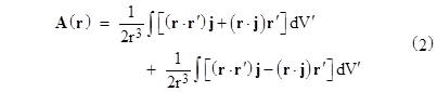
For sufficiently small r′/r we can take just these leading two terms. Also, note that the integral of the current around any stationary closed loop is zero, so the first integral in this expression vanishes identically, and hence the second term is the lowest-order non-zero term. In the second integral we can trivially replace r∙r′j with [(r∙r′)j + (r∙j)r′ + (r∙r′)j – (r∙j)r′]/2 and write the vector potential as

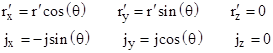
This is only approximate because we have neglected the higher order terms of the expansion in r′/r, but it becomes exact in the limit as r′/r goes to zero. We will show in full generality that the first integral in this expression identically vanishes (for any stationary distribution of current) and the second gives the desired vector potential. However, we begin by considering the special case of a closed circular loop of current in the xy plane centered on the origin. For such a loop, letting q denote an angular parameter, we can write

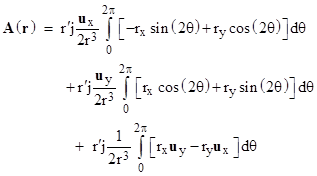
Making these substitutions into the above expression for A(r) and converting the integrals to line integrals around the loop, the vector potential for this circular ring of current is

The first two integrals (which together comprise the first integral in the previous expression) evaluate to zero, and the third gives the result

On this same basis, substituting the components of r′ and j for this circular ring in the xy plane into the definition of the magnetic moment, we get

Recall that for arbitrarily small r′ we can specify a large enough current j so that m is held constant. Thus, for this circular loop, we have

To show that this holds more generally, we return to equation (2) and assert that for any stationary current distribution the first integral vanishes identically. To show this, it suffices for our purposes to consider any number of closed current loops. (Remember that we have stipulated all the current is in a small region compared with r, and the current is stationary.) Note that j is proportional to dr’/dλ for a path parameter λ around a given loop. We can express the volume integral as path integrals around the current loops, and let x,y,z denote the components of r′, and let dx, dy, dz denote the components of dr′. Writing out the integrand explicitly in terms of the components, we find that the integral of the x component of the integrand is proportional to

Noting that d(xy) = xdy + ydz, and so on, we see that each of these integrals vanishes identically around any closed loop, and similar reasoning applies to the integrals of the y and z components.

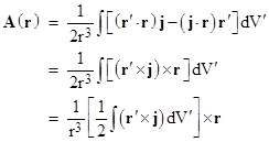
Hence we are left with just the second integral in equation (2). Making use of the well-known triple product identity, and the fact that r is constant so it can be taken outside the integral, we have

The last expression in square brackets is just the definition of the magnetic moment m, so arrive (again) at the result

which is exact in the limit as the maximum value of r′ where current is present goes to zero. (Remember that we must increase j as needed to hold m constant.)

Now, the magnetic field B(r) is the curl of the vector potential, so we have

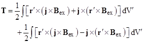
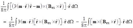
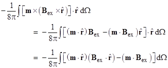
This is exact in the limit as the spatial extent of the current distribution shrinks to zero, so it applies to our idealized concept of a point-like magnetic dipole. We see that this expression is identical to the one we derived previously based on a dipole consisting of two adjacent hypothetical magnetic monopoles. Also, as Becker points out, similar reasoning leads to an expression for the torque experienced by a given Amperean dipole in an ambient uniform magnetic field that is identical to the torque that would exist for a hypothetical Coulombic dipole. From the Lorentz force law we know the force on a current element j at a given location in a uniform external magnetic field B_ex (not to be confused with the field of the dipole) is j x B_ex, so the total torque for a given distribution of current is

This can be written in the equivalent form

Again it can be shown that the first integral vanishes (for stationary current), and we can make use of the vector cyclic identity

and the fact that a x b = –b x a, to give

which is identical to the torque on a hypothetical point-like Coulombic dipole.

Since they apparently have identical fields, and they experience the same torque in a uniform magnetic field, one might think that, in the limit of point-like configurations, Coulombic and Amperean dipoles are completely indistinguishable – at least as far as their magnetic properties are concerned. However, there’s an interesting difference between these two models for magnetic dipoles that actually has an observable effect. Consider, for example, the integral of the magnetic field B of a point-like dipole within a spherical region of radius R centered on the dipole. We might just try to integrate the expression for B(r) that we derived above, but that expression contains a singularity and directional ambiguity at r = 0. On might thing that, since the volume of the region at precisely r = 0 is zero, it can’t contribute to any meaningful quantity, but remember that we increased the charges or currents to infinity as we shrank the size to zero, to give a fixed magnetic dipole moment. Likewise the limiting value of the integral of B(r) within a spherical region surrounding the charge or current need not be zero as the radius shrinks to zero. In fact, we find that it approaches a finite value. However, this limiting value is different, depending on whether we model the dipole as two adjacent monopoles or as an electric current loop.

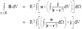
J. D. Jackson’s Classical Electrodynamics described a method of deriving these limiting values. For a magnetic field produced solely by electric current we can integrate the magnetic field B within a sphere of radius R by integrating the curl of the vector potential given by equation (1), and we can convert this to a surface integral as follows

where n denotes a unit vector normal to the surface (pointing outward). Substituting the expression for A from equation (1), we have

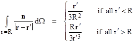
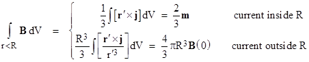
It can be shown that the angular integral is

The first case applies when all the current is inside the sphere of radius R, and the second applies when all the current is outside the sphere.

where we’ve invoked the basic law of magnetic induction in the second expression. The first expression applies regardless of how small we chose R, provided only that all the current is inside the sphere. Hence in the limit for a point-like dipole, this is the value of the integral of B at the point of the dipole, even though equation (3) for the magnetic field surrounding a point-like dipole is indeterminate at the dipole itself. So, if we agree by convention to define the value of equation (3) as zero at the origin, then we need to augment that expression by another term, making use of a delta “function”, to give the correct integral. This leads to the familiar expression

where d(r) is the three-dimensional delta function, which is zero for all r > 0, and which integrates to a value of 1 at r = 0. In contrast, if we perform a similar analysis for the field produced by a point-like Coulombic magnetic dipole, we find

We know from atomic theory that the orbital magnetic moments of atoms are produced by moving electrons, but for elementary point-like particles (such as electrons, protons, etc) that possess intrinsic magnetic moments it isn’t self-evident whether we should expect them to be of the Amperean type described by equation (4) or the Coulombic type described by equation (5). However, there is a phenomon involving the so-called hyper-fine structure interaction that seems to shed some light on this question.

The spectrum of emissions from an atom of hydrogen (for example) includes a characteristic contribution proportional to the energy between the singlet and triplet states of the 1s state of the atom. This is called the hyperfine structure interaction, and the energy difference is proportional to the coefficient of the delta function in the expression for the point-like dipoles. The coefficient +2m/3 in equation (4) implies a characteristic emission with a wavelength of 21.1 centimeters, whereas the coefficient –1m/3 in equation (5) implies just half the frequency, corresponding to a wavelength of 42.2 centimeters. In 1951 Purcell and Ewen employed a radio telescope specifically designed to observe these wavelengths, and detected the characteristic emission at 21.1 centimeters, the so-called “21 cm line”. This has been immensely valuable for astronomers, partly because hydrogen is a very common element so there is an abundance of emitting sources, and partly because radio waves at this frequency can pass through thousands of parsecs, whereas visible light is absorbed and obscured by the interstellar material the permeates our galaxy. In addition, the fact that the frequency is so precisely determined (for the rest frame of the emitting hydrogen) enables astronomers to apply the Doppler formula to infer the motions of the sources from the slight shifts in the observed 21 cm spike. Of course, the very presence of this 21 centimeter line (and the absence of a line at 42 cm) could be taken as evidence that even the magnetic moments associated with the intrinsic spin of elementary quantum particles behave (in some sense) as if they are produced by electric current rather than by magnetic dipoles. On the other hand, this shouldn’t be interpreted as meaning that the dipole moment is actually produced by a classical current.

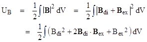
We conclude this discussion by considering the frequent claim that the expression for the magnetic field of a dipole implies a paradox when that expression is used to evaluate the energy of a magnetic dipole m in a uniform magnetic field B_ex. Consistent with the torque experienced by the dipole, we know that the magnetic energy is U_B = – m∙B_ex. However, we can also evaluate the energy of the magnetic field directly from the well-known (perhaps too well known, as we shall see) expression

Since the external field is stipulated to be uniform throughout space, the integral of B_ex² is infinite. However, only the dot product term depends on the angle between the field vectors, and since we are interested only in the change in energy with the orientation of the dipole (not the absolute value of the energy), we can omit the integrals of the other terms (even though one of them is infinite) and simply write

Without loss of generality we can assume the external field is constant in the z direction of xyz Cartesian coordinates, and we can substitute our previously derived expression for the magnetic field of the dipole, to give

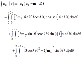
We can show that only the delta term contributes to the energy, because the other terms integrate to zero. To prove this, note that for any given r the integral of those other terms over the spherical surface is proportional to

Each of the integrals vanishes, so these terms contribute nothing to the orientation-dependent magnetic energy. Thus we are left with

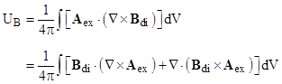
This result is surprising for two reasons, first because it apparently has the wrong magnitude and second because it apparently has the wrong sign. However, as hinted above, this is not quite right. The “well-known” expression for the energy is derived from the following expression for the energy of a current distribution j in an external field B_ex with the corresponding vector potential A_ex = (B_ex x r)/2

Using the Maxwell equation  this can be written as

The gradient of the potential is just the field, so we can replace  with B_ex. Also, using Green’s Theorem we can convert the volume integral of the second term into a surface integral on any surface surrounding a given region of space, so the energy that has been expended to produce this configuration can be expressed as a sum of (1) a volume integral over any region enclosing all the current and (2) a surface integral over the surface of that region. Thus we have

where  denotes the unit vector in the direction of r. The first term has the same form as equation (6), but we also have the additional surface integral. In some circumstances when we integrate the first term over all space we can neglect the surface integral, but only if that integral goes to zero as the size of the enclosed volume goes to infinity. In the case of a dipole in a uniform external field (presumed to extend to infinity) the surface integral does not go to zero, as can be seen from the fact that B_di is proportional to 1/r³, and A_ex is proportional to r, so the product is proportional to 1/r², and the surface area increases in proportion to r² as r increases. Hence the factors of r cancel, and, replacing A_ex with (B_ex x u_r)/2, the surface integral becomes an angular integral

The first integral vanishes identically, because we have

Therefore the surface integral is

The second term in the integrand is constant, and the angular integration gives

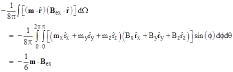
To evaluate the first term in the integrand of the previous expression we can write out the vectors in component form, noting that

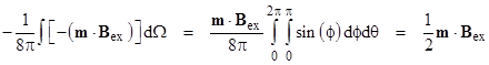
Carrying out the integeration, term by term, we find that each of the off-diagonal terms in the product of the two dot products gives an integral of zero, so only the diagonal terms contribute to the integral. Thus we have

The total surface integral is therefore (1/2 – 1/6)m∙B = (1/3)m∙B, which we add to the previous volume integral to give the total

Jerrold Franklin has given a nice explanation of where the addition (1/3)m∙B actually resides, since it is not in the space covered by the volume integral to infinity, and indeed we know the integrand of that volume integral is the correct energy density. The explanation is that some of the energy required to establish this configuration flows out through the boundary of the volume, and this flow in independent of the size of the volume, so it applies even in the limit of infinite volume. Of course, one can argue that an infinite uniform field is not realistically possible, and the ultimate static dipole field extending to infinity cannot be established in any finite length of time (due to the finiteness of the speed of light). But this analysis shows what is necessary to correctly account for all the energy in this hypothetical situation.

However, another apparent “paradox” remains. Our result has the expected magnitude, but apparently the wrong sign. It’s worth noting that we get the same answer even if we use a finite current loop for the dipole and finite sources for the external field. On the other hand, if we model the magnetic dipole as two adjacent magnetic monopoles, the same analysis shows that the delta term in the volume integral for the energy gives –m∙B_ex/3 and the surface integral contributes –2m∙B_ex/3, for a total of –m∙B_ex. Thus the Coulombic model gives us the expected result, but the Amperean model seems to give the wrong result.

The explanation for this apparent contradiction is that a magnetic dipole produced by free electric current is a more complicated entity than a dipole produced by static monopoles, and involves both electric and magnetic energy when we consider re-orienting current loops in the fields produced by other current loops. As discussed in (for example) Schwartz's "Principles of Electrodynamics", when displacing a current loop, in the presence of a magnetic field produced by one or more other current loops, we need to distinguish two different ways of carrying out the displacement, and the two different physical consequences. One might think the right way is to displace our tiny current loop while holding the currents (in all the loops) constant, and indeed this is the basis of the Amperean energy calculation described above (that leads to the wrong sign for the energy). However, holding constant current will necessarily result in a change in the flux in the loops (like tiny generators). While the flux is changing, the integral of E∙dl around the loop will not be zero, and hence the electric field will do work on the currents in the loops, and this work is in addition to the purely magnetic effect we are trying to evaluate.

Another way of carrying out the displacement is with the fluxes (not the currents) held constant. Using this method, the integral of E∙dl around each loop is automatically zero, so we do only the magnetic work. Therefore, to determine the magnetic energy of a magnetic dipole, the relevant quantity is the change in energy for a spatial displacement or re-orientation while holding constant flux, not constant current. However, it's much more straightforward to evaluate the change in energy at constant current (as we did above), so this is usually what is done, but then we make use of a remarkable theorem, which says that for a given displacement of a set of current loops, the change in magnetostatic internal energy due to carrying out that displacement at constant current is the negative of the change in energy due to carrying out the same displacement at constant flux. Thus we have

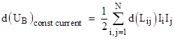
This illustrates that interaction between two (or more) current loops is more complicated than one might think. In a set of N current loops, the magnetic flux through the ith loop has a contribution to it arising from the current in each of the other loops. The magnetic flux through the ith loop is the integral of B∙n over any surface bounded by the loop (where n is the unit vector normal to the surface), and this depends not just on the current through the ith loop, but on the current through each of the loops, i.e., the flux through the ith loop is written as the sum of L_ij I_j for j = 1 to N where the constants L_ij are the coefficients of inductance. In other words, there is mutual inductance, so we do not simply superimpose two independent B fields. The coefficients of inductance are given by the double line integral of (1/|r_i - r_j|) dl_i dl_j around the ith and jth loops, and hence L_ij = L_ji. Then the overall magnetostatic energy of the system of loops is the sum of (1/2) L_ij I_i I_j for i,j = 1 to N. For example, with N = 2 loops the energy is

Now, for an incremental displacement of these loops, holding all the currents constant, only the L_ij coefficients change, while the I terms are constant, so we have

On the other hand, making the displacement at constant flux, we get the negative of this, i.e., d(U_B)_flux = –d(U_B)_current. This is exactly analogous to how, in electrostatics, the change in energy when displacing a set of conductors at constant charge equals the negative of the change for the same displacement at constant potential. In the electrostatic case, the relevant process is displacement at constant charge when determining the forces acting on the conductors, which corresponds in the magnetic case to displacement at constant flux when determining the torques acting on the current loops.

Becker also discusses this same topic. In a nutshell, we can't treat displacements of current loops by considering just the magnetic field, if the currents are held constant, because in that case the effects of mutual induction must be taken into account, and the electric field does work on the system. Becker shows explicitly that, holding the currents constant, a current loop will do work equal to the increase in the magnetic field energy, and this double expenditure is supplied by the electromotive force that must be applied during the displacement in order to maintain the constancy of the currents. On the other hand, if no electromotive force is applied to keep the currents constant, they will change in response to a displacement, but the flux will be constant. For such a displacement, the work done equals the reduction in the magnetic field energy.

One remaining point of confusion pertains to the distinction between dipoles produced by free current versus dipoles associated with magnetized materials. In the latter case we don’t have to apply external electromotive force to maintain the current. Thus there is an important difference between the energy calculations for a magnetic dipole produced by “free current” and one produced by a magnetized substance. The distinction is captured by the difference between the B and the H fields. Outside any magnetic material, B and H are strictly proportional to each other, but inside magnetic material they are quite different. The potential energy density of a magnetic field is really B∙H/2, and reduces to B²/(2μ₀) only outside of any magnetic material.

Take for example a spherical shell of uniformly magnetized material. Outside the shell the B and H fields are essentially identical, being that of a perfect dipole, for which the field energy is indifferent to orientation. Inside the sphere, there is a uniform field, but the direction of the H field is opposite the direction of the B field in this interior region. Thus, in the region that counts (inside the magnetized sphere), the relevant field is the H_di field, which points in the opposite direction of the B_di field. The reason we need to use H is that a magnetic field B is caused by two different types of currents, which are sometimes called “free current” and “bound current”. The free currents are the ones we would usually identify as electrical currents in a system, produced by hooking up a battery to a wire, or some similar method. In contrast, the “bound currents” are the ones we infer must be present in atoms comprising a permanently magnetized substance. Unlike free currents, bound currents don’t do any work, so when we perform calculations involving the energy of the magnetic field we need to distinguish between the fields produced by these two kinds of current. This is why we need to use the field energy expression based on the H field when considering magnetized objects.

Return to MathPages Main Menu