Two Envelopes

The loss at the boundary cancels all the gains in all the other cases combined.

                                                                                                      April 18, 2014

Suppose we are offered a choice between two identical-looking envelopes, each containing some amount of money, one twice as much as the other. Which envelope should we choose? From the information we’ve been given, we cannot infer that one of the envelopes is more likely than the other to contain the larger amount of money, so in this situation we have no reason to prefer one envelope over the other.

Now suppose we randomly select one of the envelopes, but before opening it, we begin to have second thoughts. Should we have chosen the other one? At this point we might be tempted to reason as follows: By switching to the other envelope we will either double or halve our money, each with probability 0.5, and therefore (according to this reasoning) it is beneficial to switch, because our expectation is increased by the factor 0.5(2) + 0.5(1/2) = 5/4. Of course, if we switch to the other envelope and apply the same reasoning, we will conclude that it is advantageous to switch back, and so on, ad infinitum.

Needless to say, this reasoning is invalid. To help explain the fallacy, let [A,B] denote the situation in which the originally selected envelope contains A and the other envelope contains B. The above reasoning assumes that for some fixed x the two equally probable alternatives after selecting one of the envelopes are [x,2x] and [x,x/2]. If this were true, it would indeed imply the expected values of the envelopes are x and 5x/4 respectively. But it is not true. For some fixed x (equal to one third of the total money in the two envelopes combined) the two equally probable alternatives are actually [x,2x] and [2x,x], so the expected value of each envelope is 3x/2, and hence there is no reason to prefer one envelope over the other (as is intuitively obvious).

The fallacy in the reasoning that led to the expectation 5x/4 for the “other” envelope was the implicit assumption that the content of the originally-selected envelope is independent of the content of the other envelope. Yes, we could let a single symbol X denote the fixed (but unknown) amount of money that is actually contained in the first envelope (regardless of which envelope has the larger or smaller amount), but by the same token we can let the symbol Y denote the fixed (but unknown) amount that is actually in the other envelope. In terms of these symbols the situation we face is unambiguously [X,Y], but this gives us no information as to which envelope contains the greater amount. All we know is that, for some fixed x = (X+Y)/3, we either have X=x,Y=2x or else X=2x,Y=x.

Notice that this analysis doesn’t depend at all on how the amounts in the envelopes were chosen, i.e., it doesn’t depend on the distribution from which the amounts were drawn, nor on whether we have any knowledge of that distribution.

But now suppose we look inside our originally selected envelope, and see that it contains (say) $16. What now?  Should we keep this money, or would it be advantageous to relinquish this envelope and take whatever is in the other envelope? Now we actually have some information that could, in some contexts, warrant some preference for one envelope over the other. In particular, if we know the distribution from which the total amount in the two envelopes was drawn, we can use our knowledge of the contents of the first envelope to determine the exact probability that the other envelope contains more.

To illustrate, suppose we are told that the amounts of money in the envelopes were chosen by first randomly selecting a number from the set (1,2,4,8,16,32,64) and then placing that many dollars in one envelope and twice that many in the other. This means the seven equally probable pairs of amounts are (1,2), (2,4), (4,8), (8,16), (16,32), (32,64), and (64,128). In this context, if we find $16 in one envelope, the other envelope is equally likely to contain $8 or $32. Thus the expected value of the other envelope is 0.5($8) + 0.5($32) = $20, so it is indeed to our advantage to switch. Similar reasoning would lead us to switch upon finding any of the values 2, 4, 8, 16, 32, or 64 in our originally selected envelope. Of course, we would also switch if we found $1, in which case we are certain to double our money. However, if we find $128 in our original envelope, we should definitely not switch.

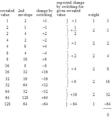
In this example the amounts of money in the envelopes are chosen based on a uniform distribution for the seven amounts 2^j with j = 0 to 6, and the result is that we should switch upon finding any amount other than $128 in the first envelope. Thus there are 14 equally likely scenarios (randomly choosing one of the seven pairs of numbers, and then randomly choosing to reveal one of those two numbers), and in 13 of those scenarios we should switch. The table below shows the 14 possible and equally probable scenarios. The numbers in the first column are the amounts in the first envelope, revealed to the player, and the numbers in the second column are the amounts in the second envelope.

The third column lists the amounts of gain (or loss) by switching to the second envelope in each of the 14 possible (and equally likely) cases. In the fourth column we’ve listed the expected amounts of gain (or loss) for each revealed value. For example, there are two cases where the revealed value is $8, and in one of those cases the value in the second envelope is $4, whereas in the other case it is $16. In the first case the player loses $4 by switching, and in the second case he gains $8. These two cases are equally likely (on the condition that the revealed envelope has $8), so they each have probability 0.5 given that the revealed amount is $8. Therefore, the expected gain for switching to the second envelope is 0.5(-4) + 0.5(8), which equals +2. The fifth column shows the weights of the conditional scenarios. This is to account for the fact that we are twice as likely to have a revealed number of (say) 64 as we are to have a revealed number of 128.

The last column in the table gives the weighted gains or losses for each revealed amount. This shows that for each revealed value except 128, switching increases our expected money by a factor of 5/4 (or 2, for the revealed value of 1), but for the revealed value of 128 switching will decrease our expected money by a factor of 1/2, which is enough to wipe out all the gains for all the other cases combined. So, even though switching is advantageous in 13 of the 14 cases, it provides no advantage at all when averaged over all 14 cases.

To make the situation even more clear, suppose we are told that the envelopes are prepared based on a uniform distribution for the values 2^j with j = 0 to one billion. One of these values is randomly selected for one envelope and then twice that amount is placed in the other envelope. Then we randomly make our initial selection, and the contents of that envelope are revealed to us. In this case there are two billion equally probable scenarios, and in all but two of them our expected money by switching is 5/4 times whatever value we see in the first envelope. Therefore, when presented with such a scenario, it is virtually certain that the revealed value will be one of the non-boundary values, and therefore the conditional expectation for switching is to increase our money by a factor of 5/4. Nevertheless, if our strategy is to always switch, regardless of the revealed contents of the first envelope, then our expected overall gain by switching is nil. This may seem surprising, given that switching is virtually certain to increase our money by a factor of 5/4. The explanation is the same as in the previous example, i.e., although the probability of finding the top-most value in the first envelope is extremely small, the penalty is large enough to swamp all the expected gains from all the other scenarios combined. So, even though the player will almost certainly find himself (after opening the first envelope) in a scenario in which switching increases his money by a factor of 5/4, the overall expected value of switching is zero. This explains why, prior to seeing the contents of the first envelope, the expected values of the two envelopes are the same, because the expectation takes into account the huge loss for the one possible case at the upper boundary of the range, even though the probability of being at that boundary is extremely small. In this respect the situation closely resembles the St Petersburg paradox, in which arbitrarily unlikely outcomes contribute significantly to the expectation because of the proportionately huge effects those outcomes would have on the results.

We’ve seen that the answer to the two-envelope problem, when we don’t know the contents of either envelope, is that the expected values of both envelopes are equal. In this case the conundrum is due to incorrectly thinking the equally probable possibilities are [x,2x] and [x,x/2] for some fixed x, whereas the actual possibilities we face are [x,2x] and [2x,x] for some fixed x. The distribution of x doesn’t matter, since we don’t know the contents of either envelope. Now, when we go on the consider the situation after the content of one envelope has been revealed, the answer becomes more nuanced, partly because it depends on the distribution, and partly because there are two components of the answer. We’ve shown above that it’s possible for the distribution of x to be such that, although the expected benefit of switching is zero when we average the conditional expectations over every possible revealed value, the conditional expectations for all but the two values – those at the boundaries – favor switching. In particular, there are distributions such that, for all but the boundary values, switching is equally likely to double or halve our money, and hence switching gives an expected benefit of increasing our money by 1/4. Furthermore, we can make the probability of encountering the boundary on any given trial arbitrarily close to zero, so that any reasonable person would be highly confident that the revealed value is not at the boundary, and therefore their expectation is improved by switching, almost regardless of the revealed value.

This might seem to re-introduce the paradox, as can be seen most vividly by imagining that the numbers x and 2x are written on opposite sides of a card, and the card is held up between two players, each of whom is asked to decide if he wants the number of dollars shown on his side of the card (which he can see) or the other side of the card (which he can’t see). According to what we’ve just said, if x is chosen from the values 2^j with j = 0 to a billion, both players would be highly confident that they should take the number on the opposite sides (assuming the utility is always proportional to the amount of money, which of course is unrealistic, but is an implicit assumption of the problem). Note that in our seven-valued example, if we neglect the cases when the player sees a boundary value (1 or 128), his expectation for the other side is exactly 5/4 of the value of the side he can see. Actually, it’s even more beneficial for a player to switch when he sees the lower boundary value of 1, so the only case that really needs to be excluded in this example is the upper boundary (although for other distributions it is the lower boundary that must be excluded, as discussed below). It might seem surprising at first that this can be true for both players, i.e., that a winning strategy for both players is to always choose the number on the opposite side of the card, excluding the cases when they see 128 (the upper boundary). However, there is nothing mysterious about this. In the table where we presented the results for the seven-valued example, notice that if we exclude the rows where 1 or 128 appear in the first column, the columns sum to 252 and 315 respectively, whereas if we exclude the rows where 1 or 128 appear in the second column, the columns sum to 315 and 252 respectively. The reciprocity is possible because the boundary cases are different for the two players. (It’s amusing to note the analogy between this and the two different simultaneities for relatively moving inertial coordinate systems according to special relativity, enabling the Lorentz transformation to be completely reciprocal.)

But how can both players benefit by switching to the number on the other player’s side of the card? Obviously for every amount that one of them gains by switching, the other loses that same amount by switching on that card. In any series of trials, limited in number so that they are unlikely to encounter the boundary, they can’t both come out ahead. The explanation is that the amounts of gain and loss vary by orders of magnitude, and cannot be expected to approach the asymptotic return until a sufficiently large number of samples have been drawn from the entire range of possible values. To illustrate with our example of 14 possible sets of numbers and arrangements, suppose we have the following four trials:  [4,2], [8,16], [32,16], [32,64]. If both players always switch, the effect of switching for the first player is -2, +8, -16, +32, whereas the effect of switching for the second player is +2, -8, +16, -32. Thus, the lead changes hands, and the size of the lead increases, on each round. The cumulative outcomes will not converge on the expected values until many more trials covering the entire range have been performed. But this requires a representative sampling over the entire range, which ensures that the boundary will be encountered a representative number of times. (This is unavoidably true, because one player’s boundary card is the other player’s most significant non-boundary card.) If the players take advantage of their knowledge of the number on their own side of the card, and refrain from switching when they are at the boundary, but switch in all other cases, they will indeed come out ahead in the long run. But if they simply switch all the time, regardless of the amount on their side of the card, they will just break even.

The reason this tends to seem counter-intuitive is because it can take so long to encounter the boundary, and we may feel that in the short run the boundary can be neglected. But in fact, as already noted, the results converge on the theoretical expectation only when the boundary is fully represented. It’s worth repeating that the boundary can be pushed as far away as we like, making it arbitrarily improbable for any given card to contain the boundary, and yet in order for the expectations to converge on their ultimate values we would need to perform enough trials so that the boundary is proportionately represented. Thus we cannot avoid taking the behavior at the boundary into account, and this fully reconciles all the expectations, disposing of the paradox.

One might think that the boundary could be eliminated by stipulating that the envelopes are prepared based on a uniform distribution for the values 2^j with j = 0 to infinity. However, this is not possible, even in principle, because there does not exist a uniform distribution over the natural numbers. Of course, it isn’t necessary for the distribution of the j values to be perfectly uniform. We could, for example, stipulate that each value of j has probability (1/3)(2/3)^j, which is a well-behaved distribution, but the mean value of 2^j (the amount in the smaller envelope) is infinite for this distribution. More generally, we could stipulate that the value of j has probability (1−q)q^j for any q, but this gives a finite mean for 2^j only if q is less than or equal to 1/2, in which case the advantage for switching disappears.

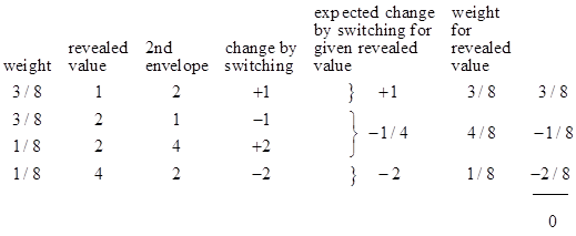
In fact, with a value of q less than 1/2, or more generally with any distribution that drops by more than 1/2 for successive values of j, we can construct a reverse paradox, in which it is almost always better to not switch. For a very simple example, suppose the amounts in the envelopes are chosen as either (1,2) or (2,4), with probabilities 3/4 and 1/4 respectively. The resulting expectations are shown in the table below.

In this case the lower boundary is the one that provides the off-setting probability, so that the overall expected change from switching is nil, even though for every case other than the lower boundary the expected change is negative. (It’s worth repeating that with these inverted distributions we can eliminate the upper boundary, but the lower boundary plays the exceptional role, so we haven’t eliminated the exceptional boundary.) Of course, with any non-uniform distribution we can not expect, even approximately, that the probabilities of doubling or halving our money are equal. Indeed this harkens back to a problem closely related to the two envelope problem that Littlewood (in his “A Mathematician’s Miscellany”) attributed to Schrodinger:

We have 10ⁿ cards of the type (n, n+l) [i.e., with n written on one side and n+1 written on the other], and the player seeing the lower number wins. Players A and B [who can each see just one side of the card] may now bet each with each other... Whatever A sees he should bet, and the same is true of B, the odds in favour being 9 to 1. Once the monstrous hypothesis has been got across (as it generally has), then, whatever number n that A sees, it is 10 times more probable that the other side is n+l than that it is n−1. (Incidentally, whatever number N is assigned before a card is drawn, it is infinitely probable that the numbers on the card will be greater than N.)

It isn’t surprising that Schrodinger was interested in such questions, because the non-commuting infinite matrices of quantum mechanics rely on precisely this kind of “monstrous hypothesis”, without which it would not be possible to satisfy the commutation relations.

So far we’ve considered only cases in which the player knows the distribution from which the contents of the envelopes were drawn, and we’ve insisted on the distribution being well defined. But the original problem statement does not specify any distribution, nor does it provide any clue as to how the amounts in the envelopes were chosen, other than the stipulation that one envelope contains twice as much as the other. As we’ve just seen, it’s easy to define distributions for which the expectations usually favor switching, or usually favor not switching, and also for which the revealed value provides significant information about the expectations. An extreme example is to choose the amounts by placing an odd number of dollars in one envelope and twice that many dollars in the other. Obviously we would always switch when shown an odd number, and never when shown an even number.

But in the absence of any information about how the amounts in the envelopes were chosen, one might think that knowledge of the contents of one envelope could tell us nothing about whether the other envelope contains twice or half that amount, and hence we are thrown back to the symmetrical case, with no basis for preferring one envelope over the other, even after we’ve seen the contents of one of them. This is almost true, but with a caveat that there exist strategies that do, in principle, give us some non-zero advantage in deciding whether to switch, based on knowledge of the contents of the first envelope – although the amount of the advantage may well be vanishingly small.

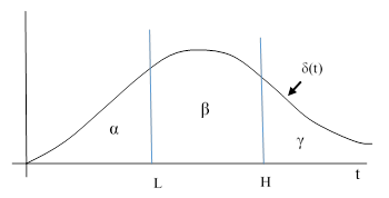
One such strategy is as follows: After seeing the contents of the first envelope, we will randomly select a number from a well-defined density distribution δ(t), and make our decision about whether to switch as if the randomly selected number was the unknown contents of the second envelope. In the figure below the numbers L and H denote the values of the low and high amounts in the envelopes. We select one of these envelopes at random, and open it. Then we randomly select a number from the density distribution δ(t). If the randomly selected value of t is greater than our revealed value, we will switch, otherwise we will not switch.

The probability of initially choosing the envelope with L is 0.5, and likewise for the envelope with H. If we initially choose the L envelope and expose its contents, our strategy will lead us to the correct decision (i.e., switch) with probability β + γ, and will lead to the wrong decision (i.e., don’t switch) with probability α, because these are the probabilities of our randomly chosen value of t to be greater than or less than L, respectively. On the other hand, if we initially choose the H envelope and expose its contents, our strategy will lead us to the correct decision (i.e., don’t switch) with probability α + β, and will lead to the wrong decision (i.e., switch) with probability γ, because these are the probabilities of our randomly chosen value of t to be less than or greater than H, respectively. Hence with this strategy the probability of ending up with the higher amount is0.5(β + γ) + 0.5(α + β), and the probability of ending up with the lower amount is 0.5(α) + 0.5(γ). The difference between these two probabilities is simply β, which is always greater than zero for any continuously positive density distribution.

Of course, this strategy provides a significant benefit only if the density function δ(t) has significant area under the curve between L and H. Our drawing above is for the most fortuitous case when L and H straddle the highest density range of the function, but in general we would not expect this to be the case, unless we have some prior knowledge that L and H are preferentially in that range. As already noted, there is no uniform density over the reals, so we come back again to the requirement to make use of some knowledge of the distribution of the L and H values. If they were drawn from an extremely flat distribution, such that they could (and usually would) be huge numbers, then L and H would almost certainly be far away from the region where δ(t) has any significant value, and hence β would be virtually zero and the strategy would provide no significant benefit. (For a related discussion, see Choice Without Context.) Note that we cannot chose our density function based on the initial revealed value, we must agree in advance to use the same density function regardless of the revealed value.

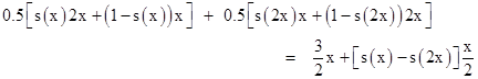
Notice that the above strategy essentially just amounts to defining a probability function for switching or not switching, based on the revealed value. We can streamline the approach by simply defining a probability function s(r) as the integral δ(t) over the appropriate range, and using this function to determine our choice. In other words, after selecting one of the envelopes at random and determining its contents, r, we then decide whether to switch by a random process such that the probability of switching equals s(r).  This is equivalent to sampling from the density distribution δ(t). For example, if we define s(u) = e^−u, and if the revealed value is one dollar, we will switch with probability e⁻¹ = 0.369, whereas if the revealed value is two dollars we will switch with probability e⁻² = 0.136, and so on. There is a 0.5 probability that the revealed number is x (where x is one third of the total in the two envelopes), and a 0.5 probability that it is 2x. In the first case we will switch with probability s(x) and not switch with probability 1−s(x). In the second case we will switch with probability s(2x) and not switch with probability 1−s(2x). Therefore, our expected value is

Provided our density function s(u) is strictly decreasing, so that s(x) is greater than s(2x) for all positive values of x, this strategy gives us an expected result greater than 3x/2. Of course, with s(u) = e^−u and x equal to (say) 100, the benefit of this strategy is already vanishingly small, so, as noted above, the practical utility of this strategy is dubious, unless we can exploit some knowledge of the distribution of the amounts in the envelopes.

Note also that the above equation confirms that if s(u) is constant (for example, if we always switch, or if we never switch, or we switch with any fixed probability, independent of the revealed number r), then the expected value is 3x/2. Thus the outcome is indifferent to our choice of envelopes, as one would expect in the absence of any information about how the envelopes were prepared. Needless to say, in reality we would always have some information, since the total amount of money in the world is limited, etc., so when the puzzle poser insists that the amount of money in the envelopes is completely arbitrary, we know we are being asked to consider an unrealistic scenario.

By the way, people occasionally try to “resolve” the two envelopes “paradox” by noting (correctly) that the choice of whether to switch envelopes does not affect the total amount of money in both envelopes, it affects only the fraction of the total that the player receives. Also, it’s easy to see that the expected fraction is the same, whether the player switches or not. Given that one of the envelopes is opened to reveal x, we know the other envelope contains either x/2 or 2x, and in suitable circumstances the conditional probability is 0.5 for each of these alternatives. In these circumstances, switching does indeed give an expected value of 5x/4, but the paradox resolver thinks it must not, because he mistakenly thinks it would lead to perpetual exchange, since he fails to realize that there is no well-defined distribution that would always give a conditional probability of 0.5 for each alternative after the first number has been revealed (as explained previously). So, the resolver mistakenly thinks the expectation must be indifferent to the choice of envelopes in this condition. To justify this, and thereby resolve the paradox (as he thinks), he reasons as follows:  Prior to seeing the contents of one envelope, we know the two possible situations are [x,2x] and [2x,x], both of which have the same total amount of money (3x) in the two envelopes combined. Once we reveal the contents of the first envelope, called x, we may consider the two situations [x,2x] and [x,x/2] (which the resolver mistakenly thinks are always equally probable), but these do not have the same total amount of money. The first has a total of 3x, whereas the second has the total 3x/2. Whether we stay with x or switch, we have 0.5 probability of having 2/3 of the total, and 0.5 probability of having 1/3 of the total. Therefore (so the resolver argues), there is no reason to prefer one envelope over the other in this condition. The fallacy of the argument is that “the total” refers to two different things. Gaining 1/3 of a larger total outweighs losing 1/3 of a smaller total, which of course is precisely why the conditional expected value of switching actually is 5x/4 in this condition. Hence this argument is invalid. The actual explanation of the two envelope problem is as discussed previously.

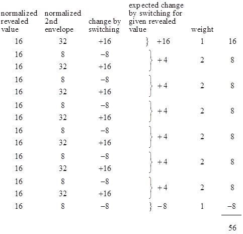
From a realistic standpoint there is an obvious caveat to all of this:  The actual utility of amounts of money on the order of 2^{1,000,000,000} dollars is questionable (to say the least). With a distribution of values 2^j with j = 0 to a billion as described previously, the player will almost certainly be faced with an amount of money (in the initially selected envelope) that is many orders of magnitude greater than all the money in the world. We might try to remedy this defect by changing the game slightly: Instead of containing actual money, each envelope might contain just a slip of paper with the number written on it, with the understanding that when the player opens the first envelope the units will be defined such that the content in the first envelope is worth, say, $1000. This does indeed result in a game where the strategy of always switching is beneficial, regardless of the revealed number, as we can see by considering again our previous example of just powers of two up to 128, normalized so that the first envelope is worth $16, as shown in the table below.

Thus, by scaling all the numbers based on the contents of the first envelope, the expected value of the second envelope is actually increased. (We could still make an exception for the case when the revealed number is 128, but it isn’t necessary.) This may seem surprising at first, because the envelopes are a priori symmetrical, with the same distribution of raw values, with the same overall sums. Nevertheless, when we normalize all the values so that the value in the first envelope is $16, the average normalized value in the second envelope is $20, whereas if we scale the numbers to make the contents of the second envelope equal to $16, the average value of the first envelope is $20. But this isn’t mysterious. Consider the simple case of just two possibilities, [2,1] and [1,2]. These are perfectly symmetrical. The sum of the first arguments of these pairs is 3, as is the sum of the second arguments. But if we scale each pair so that the first argument is 2, we have [2,1] and [2,4], so the sum of the first arguments is 4 but the sum of the second arguments is 5. Similarly if we scale each pair so that the second argument is 2, we have [4,2] and [1,2], so the sum of the first arguments is 5 and the sum of the second arguments is 4.

Since, in this normalized game, it is unambiguously advantageous to always switch, regardless of the revealed number in the first envelope, one might think this leads us back to the paradoxical conclusion that it’s beneficial to switch even without revealing a number, i.e., the perpetual exchange paradox. However, this is not the case, because without opening an envelope we have not carried out any re-scaling, so the expectations remain symmetrical. Indeed, if we stipulate that we will scale the contents of our selected envelope to (say) $16, regardless of the number, then the indifference of our choice of envelopes (prior to opening either envelope) is obvious. But once we have opened an envelope and established the scale factor based on the number that we find, the average value of the other envelope becomes greater by a factor of 5/4 due to that re-scaling, and this is true regardless of which envelope we initially choose.

In this normalized game we could actually do a bit better than 5/4 if we switch on every raw revealed number except when the revealed number is 128. Obviously the conditional expectation for the other envelope is lower in this particular case. However, the magnitude of the normalized loss if we choose to switch in this case is small enough that, considering the low probability of encountering this case, it does not greatly affect the overall benefit of always switching. This is in contrast with the un-normalized game, in which the loss in the boundary case cancels all the gains in all the other cases combined.

Return to MathPages Main Menu