Weibull and Lightning

Suppose a system is designed to be immune to lightning strikes, but the features that provide the protection against lightning can fail, with a time-dependent rate λ(t). If a system’s protection features are failed, a lightning strike will result in complete failure of the system. Let σ denote the rate of occurrence of lightning strikes (of sufficient intensity to cause system failure if the protection features are failed). Also, the system’s protection features are checked periodically, and if found to be failed they are restored to their “new” condition. We will represent this inspection/repair by stipulating that units with failed protection features are repaired at a rate μ = 2/t_I where t_I in the inspection interval. (At the end of this note we evaluate the system using discrete repairs, and compare the results with those obtained using the continuous repair model.)

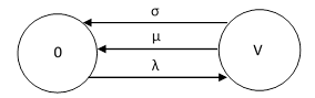
If the function λ(t) were constant, we could represent this scenario by a trivial Markov model as shown below.

State “0” has functional lightning protection, and state “V” has failed protection features, so it is vulnerable to a lightning strike. As always, for the steady-state model, the complete system failure (represented by the σ transition) feeds back into the full-up state. The rate of complete system failure is σP_V where P_V is the probability of state V. The system equation is λP₀ = (μ+σ)P_V with the normalizing equation P₀ + P_V = 1, from which is follows that the rate of complete system failure is

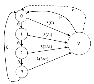
However, for our problem the function λ(t) is variable, so this simple approach is not applicable. Strictly speaking, a transition with variable rate is not Markovian, but we can represent it as the limit of a sequence of Markov models in which State 0 is split into a time-ordered sequence of sub-states, with each sub-state containing the systems of a certain age. In these models, the transition rate from each sub-state is constant, so the models can be solved using ordinary Markov model techniques. We can then evaluate the results in the limit as the sequence of sub-states becomes infinite, yielding the exact answer for the continuously variable transition rate. (For a related discussion, see the note on Markov Models with Aging Components.)

To illustrate, we will split State 0 into four sub-states, representing four spans of time in the overall life T of a system, as shown in the figure below.

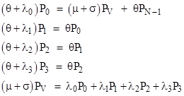
where θ = 1/Δt and Δt = T/3. (More generally, if we split up the original State 0 into sub-states 0 to N, we would set Δt = T/N.) Letting λ_n denote λ(nΔt), the steady-state system equations can be written as

along with the normalizing relation

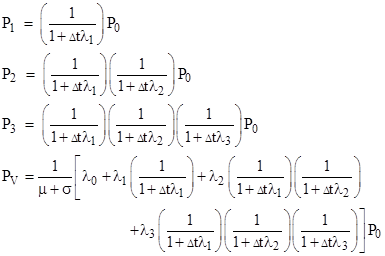
From the system equations we get

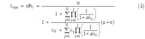
We can then insert these expressions into the normalizing equation, solve for P₀, and then substitute this value into the expression for P_V. This analysis immediately generalizes to sub-states from 0 to N, leading to the system failure rate

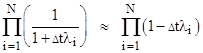
Clearly if λ(t) is constant, this reduces to equation (1) as expected. This equations can be used to compute the desired result by setting N to an arbitrarily large value (and recalling that Δt = T/N), but we might prefer to have a more explicit expression for the limit as N goes to infinity and Δt goes to zero. To evaluate this limit, we first consider the products

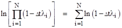
This relation becomes exact in the limit as Δt approaches zero. The natural log of this product can be expressed as the summation

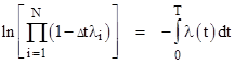
Taking just the first term of the expansion for the natural logs (which, again, becomes exact in the limit as Δt approaches zero), and converting the summation to an integration, we get

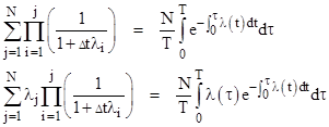
Likewise the products from i = 1 to j for j ranging from 1 to N are given by replacing T with a parameter τ ranging from 0 to T. The sums of the products can similarly be reduced to integrations, leading to the limiting relations

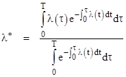
These quantities both go to infinity as N increases, so the additive constants in (2) drop out. Thus, inserting these expressions into (2) and canceling the factors of N/T, we get the system failure rate in the continuous limit:

where

Equation (3) is formally identical to (1), except that we replace the constant failure rate λ with the effective failure rate λ^*, the latter being a weighted mean of λ(t) over the life of the system.

If the loss of lightning protection has a Weibull failure rate, the function λ(t) is of the form

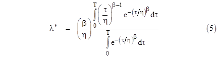
where β is the shape parameter and η is the scale parameter. If β is greater than 1, signifying a wear-out characteristic such that the failure rate increases with time, we can insert this into the expression for the effective failure rate to give

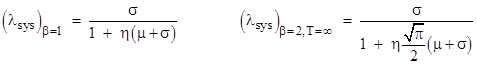
Notice that if β = 1, which signifies a constant failure rate, this expression reduces to λ^* = 1/η as expected, bearing in mind that the scale factor η corresponds to 1/λ for an exponential distribution. On the other hand, if β = 2, corresponding to the case of a linearly increasing failure rate, the expression for the effective failure rate in the limit as T goes to infinity (which is the conservative assumption) can be evaluated in closed form to give

Often the values of β for relatively mild wear-out characteristics are in the range from 1 to 2, because for values greater than 2 the rate increases exponentially. Therefore, the behavior of many systems can often be bounded between these two cases. As an example, consider the case

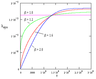
The figure below shows the system failure rate as a function of system life T for various values of β.

Just to cite one specific case, with β = 1.6 and T = 7000 we have λ_sys = (1.244)10⁻⁵. This agrees with the discrete formula in the limit as N increases.

Not surprisingly, each curve approaches an asymptotic value as T increases. It’s conservative to assume infinite life, rather than attempting to take credit for the fact that a unit may be removed from service (for some other reason) before it fails. For any value of β between 1 and 2 the asymptotic system failure rates are bounded by the two values

In the preceding discussion we represented the periodic inspection/repair at intervals t_I by a continuous transition with constant rate 2/t_I. This is quite suitable for cases where the rate of entering the failure state doesn’t change much over the duration of any single interval. On the other hand, one might question the suitability of this representation in cases with very long inspection/repair intervals, during which the the rate of entering the failed state may vary significantly. With a Weibull distribution (with β > 1) the failures are more frequent toward the end of an interval, so the mean time to repair of a failed system will be somewhat less than 2/t_I. To assess the degree of approximation introduced by the use of the continuous transition model in such cases, consider a system with a life of 96000 hours and an inspection interval of 24000 hours. Suppose the system contains 5 fasteners, and if any one or more of those fasteners fails, the system is vulnerable to a severe lightning strike, and the rate of occurrence of such strikes is σ = (8.85)10^-7 per hour. Each fastener has a Weibull failure characteristic with η = 10⁷ and β = 1.6. One very simple and conservative approach would be to assume each fastener has a constant failure rate equal to the value of λ(96000), which is the maximum possible failure rate of a fastener over its life. Inserting the values of η and β into equation (4) with t = 96000 we get (9.85)10^-9 per hour, and since there are 5 fasteners, this gives a total rate of λ_max = (4.93)10^-8 per hour. Using this value for λ and using the continuous repair model with μ = 2/24000 = (8.33)10⁻⁵, equation (1) gives λ_sys = (5.09)10⁻¹⁰. For a less simplistic approach, taking credit for the fact that the failure rate is less than the maximum value during most of the system’s life (i.e., accounting for the fact that the Weibull distribution begins with a zero rate and increases with time), we use equation (5) to give the effective failure rate for a single fastener of (6.16)10⁻⁹ per hour, so for the five fasteners we have λ^* = (3.08)10⁻⁸ per hour. Using this value, equation (3) gives λ_sys = (3.18)10⁻¹⁰ per hour.

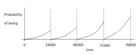
Now, to analyze this same system using a discrete representation of the repairs, we first note that the repair rate is two orders of magnitude greater than the rate of lightning strikes, so we can accurately approximate the probability of being in the vulnerable state by neglecting the lightning strikes, and simply considering a system with a Weibull failure distribution and discrete periodic repairs (neglecting lightning strikes). Given a life of 96000 hours with inspection/repair every 24000 hours, we see that the life is divided into four segments, and the probability of a system being failed at the beginning of each segment is zero, as depicted below.

During each interval, the probability of being vulnerable is simply the integral of the effective density function. Let P₁ denote the probability at the end of the first interval, P₂ the probability at the end of the second interval, and so on. We know the density distribution during the first interval is simply the standard Weibull density

With this we can compute the probability of being in the vulnerable state at the end of the first interval

where τ = 24000 is the inspection/repair interval. The density function during the second interval is the weighted average of the density functions for the two possibilities, i.e., either the system was found failed at the end of the first interval or it was not. If it was found failed at time τ, then it was restored to the initial condition, whereas if it was not found failed it continues to age using the original density. Thus the density function for the second interval is

where the time parameter t is here taken to be zero at the beginning of the second interval. With this we can compute the probability of being in the vulnerable state at the end of the second interval as

By the same reasoning as before, the density function for the third interval (now taking t = 0 at the start of the third interval) is

from which we can compute the probability of being vulnerable at the end of the third interval as

Lastly, the density function for the fourth interval (again taking t = 0 at the start of the interval) is

Written explicitly in terms of the δ₁(t) function, this is

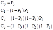
where

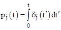
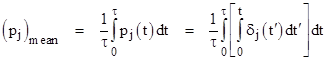
We can now compute the mean probability of being in the vulnerable state over the entire life of the system. It is simply the average of the mean probabilities over each of the four intervals. Letting p_j(t) denote the probability in the jth interval (with t = 0 at the start of the interval), we have

and the mean probability over that interval is

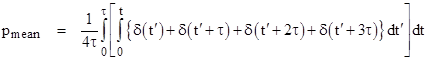
The overall mean is therefore

Inserting the values of the parameters for our example, this gives p_mean = (6.922)10⁻⁵ for a single fastener, so for one or more of the five fasteners to be in the vulnerable state we multiply this by 5 to give the probability (3.46)10⁻⁴. Multiplying this by the rate of lightning strikes, σ = (8.85)10⁻⁷ we get the rate of total system failure λ_sys = (3.06)10⁻¹⁰. This is quite close to the value of (3.18)10^-10 given by the Markov model based on continuous repairs.

By the way, since the failure rate is so low in this example, it is very unlikely that any fasteners will be found failed at any inspection, so we could simplify the calculation by simply assuming no failures, and on this basis the mean probability can be given explicitly in terms of the basic Weibull density as

This gives the result p_mean = (6.923)10⁻⁵, which is nearly indistinguishable from the exact value.

Return to MathPages Main Menu