Quasi-Eigen Systems

In a previous note we discussed the equivalence between eigenvalues and eigenvectors, and briefly considered the mapping between the normalized components of an eigenvector and the ratios of the components (i.e., eigenvalues) of that same vector. In either of these interpretations, only the ratios of the components are of significance, not their individual absolute values. However, since observations are not arbitrarily re-scaleable – at least not on the smallest scales – it’s interesting to consider the possibility that the individual components have absolute significance. There is a definite absolute scale associated with the existence of a minimal action greater than zero, i.e., a finite quantum of action, characterized by Planck’s constant h. To accurately represent physical phenomena, perhaps we ought to replace the 0 in equation (3) of the previous note with a vector of magnitude h, which we will denote as h. Having done this, the equation takes the inhomogeneous form

We call this a pseudo-eigen system. Now, assuming the matrix inside the parentheses is not singular, we could simply multiply both sides by the inverse of that matrix to give the unique solution for x, but this corresponds to the trivial x = 0 solution in the traditional formulation, except this solution will be on the order of h rather than 0. Hence this still represents a kind of trivial null solution, whereas (just as in the traditional case) the equation also possesses non-trivial solutions, provided the combined matrix on the left side satisfies a certain condition. Specifically, there will be non-trivial solutions x provided the determinant of the combined matrix is on the order of h. Thus we require

To give a simple illustration, consider the two matrices

The condition for non-trivial solution is

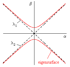
If the right hand side were zero, we could divide through by β², and this would just be the characteristic equation with two roots, representing the two eigenvalues of the system. But since the right hand side is not zero, this equation gives a surface, which we will refer to as an eigensurface. In this simple example the surface is a conic locus as illustrated in the figure below.

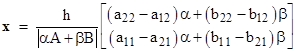
The solution x is of the form

For any point of the (α,β) plane (other than the origin) we have a solution, but since h is extremely small, the solution components will be correspondingly small unless the determinant is on the same order of magnitude as h. The eigensurface represents the locus of points on the (α,β) plane where the determinant equals h, so the leading factor in the expression for x is unity. However, the components of the solution must still be extremely small because α and β are extremely small on the eigensurface, except where the eigensurface approaches the original eigenvalues. On those asymptotes (and only there) we can make α and β arbitrarily large, but of course they must maintain essentially a constant ratio, which approaches the traditional eigenvalue the further we are from the origin. In that case the components of x approach a constant ratio to each other, i.e., they approach the traditional eigenvector.

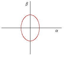
The eigensurface has several interesting features. It provides a continuous path from one eigenvalue (asymptote) to the other, but it also consists of two disjoint branches. Which pairs of asymptotes are connected depends on the particular conic that describes the locus. The hyperbolic nature of the locus is a consequence (in ordinary quantum mechanics) of the stipulation that the eigenvalues of observable operators are purely real. If h is zero (as it is traditionally taken to be), the discriminant of the characteristic equation must be positive, and hence the conic when h is non-zero is a hyperbola. However, since h is non-zero, it is no longer necessary to require a positive discriminant (so observable operators need not be Hermitian), since we can get real eigenvalues even for characteristic equations with negative discriminants. Thus we can allow for elliptical eigensurfaces as depicted below.

Of course, the solution vectors x for such systems are necessarily extremely close to null, since there are no asymptotes extending far from the origin. If h is sufficiently small, we might never notice the existence of such systems. The potential for parabolic systems is also intriguing, as they would be single-valued but allowing for solutions vectors of arbitrary size, and those vectors would not have components in constant proportion, since the parabola is not asymptotic to any fixed rays from the origin.

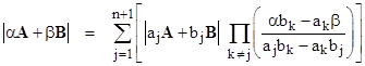
In general the degree of the eigensurface equals the order of the system. For two square matrices A and B of order n, we can express the determinant |αA+βB| in terms of the determinants |a_jA+b_jB| with j = 1, 2, …, n+1, where the (a_j,b_j) are n+1 independent “basis points” of the α,β plane. The relation can be written in the form

Equation (3) was written using the basis points (1,0), (0,1), and (1,1), but if we happen to know the n ordinary eigenvalues (μ_j,ν_j) such that |μ_jA+ν_jB| = 0 we could use them as n of the required n+1 basis points. (Of course this can be done only if there are n distinct eigenvalues.) We can then freely select just one more basis point, in terms of which to express the eigensurface equation. In doing so we must take care to preserve the scale factor, since ultimately we are setting a determinant not to 0 but to h. The characteristic equation giving the ordinary eigenvalues doesn’t contain the scale information, since only the ratios are important, so we can’t simply identify the characteristic polynomial with the determinant. Writing the ordinary characteristic equation in the symmetrical form

we have

for arbitrary constants k₁ and k₂ (not both equal to zero), and hence we can write the equation of the eigensurface as

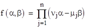
Naturally we can combine the “quantized eigen problem” with the generalization to multiple partitions discussed previously to represent interactions involving more than just two systems. It can certainly be argued that the conventional focus on purely binary interactions is not theoretically justified. If indeed there are “measurement” interactions involving (say) three systems, the relevant equation might be expressible in the form

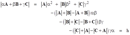
for observables A, B, and C. If the matrices are of order two, the eigensurface would then be given by

This is the equation of a quadric surface in the three-dimensional space of α,β,γ.

The key distinctions between systems described by an equation such as (4) and those described by an equation such as (5) in the previous note is that the former involves an absolute scale, so it’s important to correctly define the absolute magnitudes (not just the ratios) of the coefficients of the polynomials defining the characteristic solutions. Thus its useful to understand the form of the expressions for those coefficients. Consider the three-partition system of order n, for which we have the determinant

where m_i,j are the components of M, and σ represents a permutation [σ₁,σ₂,…,σ_n] of the indices 1 to n, and S is the set of all such permutations, and s(σ) is either +1 or -1 accordingly as the permutation σ is even or odd. In this example we make the substitutions

where a_i,j, b_i,j, and c_i,j are the components of A, B, C respectively, and we get a homogeneous polynomial of degree n in the parameters α,β,γ. Thus for some column vector R we have

where

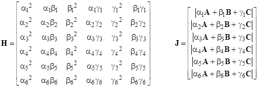
The components of R can be found by choosing 6 independent basis points (α_j,β_j,γ_j) with j = 1, 2, …, 6, and solving the system of equations

where

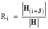
Thus letting H_(i=J) denote the matrix H with the ith column replaced with J, we can write the components of R explicitly as

We also have R = H⁻¹J, so we can express the desired determinant as a linear combination of the “basis determinants” (i.e., the components of J) by substituting into (5) to give

where K = UH⁻¹. Hence we have KH = U, and letting H^(i=U) denote the matrix H with the ith row replaced with U, the components of K can be written explicitly as

The concept of quasi-eigen problems, according to which the determinant of the system is set not to 0 but to the (small) finite value h, might provide an alternative representation of quantum mechanics. It would be interesting to determine the correspondence between these quasi-eigen systems and classical Poisson brackets as well as their analogs in quantum mechanics.

Return to MathPages Main Menu