Linear Fractional Space-Time Transformations

The preferred systems of space-time coordinates, both in Newtonian mechanics and in special relativity, consist of those in terms of which the motions of objects are as simple and symmetrical as possible. Although we have no right to expect, a priori, any degree of simplicity, the scientists of the 17th century discovered that there are in fact coherent systems of coordinates in terms of which the space coordinates of free particles are simple linear functions of the time coordinate, and in terms of which the time-derivatives of the space coordinates of two identical and initially stationary particles inter-acting with each other acquire equal and opposite values in equal times. So important is this class of coordinate systems as an organizing principle for the understanding of physical phenomena that they tend to be regarded as the “true” measures of space and time, and the special properties that characterize natural motions in terms of such coordinate systems are regarded as “the laws of motion”, which Newton attempted to formalize in the Principia. He did this by defining the “quantity of motion” of an object as the product of the object’s velocity and its “quantity of matter” (i.e., the object’s mass), and then asserting that the total quantity of motion for all objects is constant. In modern terms this expresses the conservation of momentum. When combined with a suitable definition of “force” to correlate changes in the quantities of motions of individual objects presumed to be interacting with each other, this entails all three of Newton’s laws. Since the definition of the preferred systems of coordinates is based on the properties of inertia, they are called inertial coordinate systems.

It’s worth noting that the term “inertial coordinate system” can be somewhat misleading, because the word “inertial” is sometimes used as a synonym for “unaccelerated”, whereas an inertial coordinate system must satisfy more conditions than simply being unaccelerated. In particular, the assignment of the time coordinates to separate spatial locations must be such that inertia is isotropic as well as homogeneous. It might be better to refer to coordinate systems in which inertia is both homogeneous and isotropic as “inertia-based coordinate systems”, to distinguish them from simply unaccelerated systems. Unfortunately the terminology is too firmly established to be changed, so there seems to be no way of removing this perpetual source of confusion between systems that are merely unaccelerated, and the systems discovered by Galileo and Newton, in terms of which inertia is homogeneous and isotropic (so that the explicit laws of motion take their simple symmetrical form).

The existence of even one system of inertial coordinates (in the full sense of homogeneous and isotropic inertia) is surprising, but in fact we find that there seem to be infinitely many such coordinate systems. This realization originally emerged from considerations of the Copernican model of the solar system, and the attempts to rationalize how the earth could be moving at high speed around the sun, without us having any sensation of motion. From this came the principle of relativity, according to which, for any object in any state of motion, there exists an inertial coordinate system (in the full sense) in terms of which that object is instantaneously at rest. The question then arises as to how two mutually moving systems of inertial coordinates are related to each other. It’s an interesting exercise to see how far we can go towards determining this relationship (i.e., the transformation from one system of inertial coordinates to another) from “first principles”. Prior to 1905 it was generally assumed that this relationship was trivial – a misapprehension due mainly to the lack of clarity as to the full definition of inertial coordinate systems. Only when all the intrinsic attributes of the coordinate systems used by Galileo and Newton are taken into account (along with the principle of relativity) can we proceed to consider the relationship between such systems.

Every derivation of the transformation between relatively moving inertial coordinate systems includes at some point the assertion that the transformations must be linear, i.e., of the form

where x₀ denotes the time coordinate and a_i through e_i are constants. This is certainly a plausible proposition, because a Lorentz transformation by definition represents a mapping between two systems of space and time coordinates, for each of which the space coordinates of a free particle are linear functions of the time coordinate. In some superficial treatments of the subject this is presented as sufficient reason for asserting that the transformation between two such coordinate systems must also be linear. For example, D’Inverno says

Since straight lines get mapped into straight lines, it suggests that the transformation between the frames is linear and so we shall assume [that the transformation is linear]…

Interestingly, Einstein began his derivation in 1905 as if he didn’t intend to take linearity of the transformation as an assumption, because he introduced the transformed time coordinate τ as an arbitrary function τ(x,y,z,t) of the original coordinates, and he even continued to write out the partial derivatives ∂τ/∂x, ∂τ/∂t, and so on, for about the first page. Only then did he replace these partials with constants, which he said is justified “since τ is a linear function”. No proof of this assertion is presented. Two years later he gave a slightly more refined derivation in a review article. Here he at least sketched an argument in support of the claim of linearity:

Right off, we can state about these equations that they must be linear with respect to these variables because this is required by the homogeneity properties of space and time.

This certainly conveys a sense of the argument, but it isn’t rigorous, since he never identifies “the homogeneity properties of space and time”, nor does he explain why those properties imply that the transformations must be linear. In an unpublished manuscript written around 1912 he repeated essentially the same statement, followed by some elaboration:

The functions that are being sought … must be completely linear functions... We demand this in order to preserve the homogeneity properties of physical space. If one did not make this assumption, then bodies that are at rest, congruent, and identically located with respect to S' would be differently shaped or located when referred to S; or clocks that are at rest and identically constructed with respect to S' would have different or time-dependent rates when referred to S. This will become clear later on, when we discuss the physical meaning of the Lorentz transformation.

Unfortunately this elaboration invokes the “rates of clocks”, which in special relativity represent the invariant proper times along the worldlines of clocks according to the Minkowski metric, and which already entails the Lorentz transformation. We can’t legitimately invoke any concept of proper time (or proper distance) to derive the Lorentz transformation, because we don’t have at our disposal the concepts of proper time or proper distance until we have the Lorentz transformation. At the start we have only the coordinate variables, and there is no a priori relationship between these coordinates and the rates of physical clocks. Nor are we even justified at this point in assuming that the coordinate transformation is consistent with any unified metric or pseudo-metric. As Einstein says, his justification for linearity “will become clear later on, when we discuss the physical meaning of the Lorentz transformation”. This is an admission that the justification is not clear at this stage, and that in effect he justifies linearity by the fact that it leads further on to a successful theoretical structure with physical meaning.

It’s worth noting that Einstein’s own derivations of special relativity began by taking “clocks” and “measuring rods” as primitive entities, but he admitted that this was an objectionable approach.

It is striking that the theory introduces two kinds of physical things, i.e., (1) measuring rods and clocks, (2) all other things, e,g., the electromagnetic field, the material point, etc. This, in a certain sense, is inconsistent; strictly speaking, measuring rods and clocks should emerge as solutions of the basic equations (objects consisting of moving atomic configurations), not, as it were, as theoretically self-sufficient entities.

He goes on to claim that, despite the obvious inconsistency of this approach, it was justified at the time, because “the postulates of the theory are not strong enough” to serve as the basis for a theory of measuring rods and clocks. However, it can be argued that this was a misapprehension, because the postulate of inertial coordinate systems, entailing both homogeneity and isotropy for the behavior of primitive material points (for example) when expressed in terms of such coordinates, actually is strong enough to support the derivation of the Lorentz transformation, without the need for introducing measuring rods and clocks as primitive entities. The principle of inertia, as employed by Galileo and Newton, already contains an unambiguous definition of distant simultaneity, so there is no need to invoke (for example) “slow clock transport” or synchronization by light rays to establish this physically.

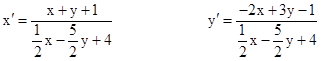
One might think that the necessity of linearity for the space-time transformations between two inertial coordinate systems – which must by definition map straight lines to straight lines – is so obvious that it’s a pedantic waste of time to dwell on the justification. However, this seemingly obvious necessity is actually false, unless we make at least one further stipulation. The most general form of space-time transformation that maps straight lines to straight lines is a linear fractional transformation

where the coefficients are constants. This system of equations has a unique inverse, and clearly if a locus of points satisfies the straight line condition

in terms of the primed coordinates, then we can substitute the preceding expressions into this equation and clear the denominators to show that it satisfies a similar straight line condition in terms of the unprimed coordinates. Thus pure linearity of the space-time transformation does not follows simply from the requirement that it map straight lines to straight lines.

Of course, the linear fractional transformations can be ruled out on other grounds. Notice that the denominator vanishes along one particular line, and hence the transformed coordinates of the points on that line are infinite. Also, the denominator is positive on one side of this “null line” and negative on the other, so for any continuous path whose coordinates cross this line, the transformed coordinates of that path go to (say) positive infinity as it approaches the line, and then discontinuously jump to negative infinity as it crosses the line. Therefore, to rule out the linear fractional transformations, we need only stipulate that the transformation must map finite coordinates to finite coordinates, or that it maps continuous sequences of coordinates to continuous sequences of coordinates. This has been recognized since the early days of relativity, as can be seen in Pauli’s 1921 encyclopedia article, where he says

All writers start with the requirement that the transformation formulae should be linear. This can be justified by the statement that a uniform rectilinear motion in K must also be uniform and rectilinear in K’. Furthermore it is to be taken for granted that finite coordinates in K remain finite in K’. This also implies the validity of Euclidean geometry and the homogeneous nature of space and time.

Thus Pauli rules out linear fractional transformations. The last sentence is interesting, because where Einstein had argued that the homogeneity of space and time implies linear transformations, Pauli asserts that the linearity of the transformations implies the homogeneity of space and time. Rindler gives an even more explicit explanation of how we arrive at the linearity requirement.

First, this relation must be linear—as is, for example, the Galilean transformation. This follows directly (though not trivially) from the definition of inertial frames: only under a linear transformation can the linear equations of motion of free particles in S go over into linear equations of motion also in S′. Actually, this requirement by itself only implies that the transformations are necessarily projective, i.e., that the S′-coordinates are ratios of linear functions of the S-coordinates, all with the same denominator. However, if we reject, for physical reasons, the existence of finite events in S which have infinite coordinates in S′, then the denominator must be constant, and thus the transformation linear.

Few people would quarrel with any of the stipulations that rule out linear fractional transformations, and hence it is generally agreed that the simple linearity of the transformations between inertial coordinate systems does indeed follow from quite basic principles.

However, as Rindler says, it is not trivial to formally prove that the linear fractional transformations are the most general transformations that map straight lines to straight lines. We could argue that the required mappings must be one-to-one, which immediately rules out functions of higher than the first degree. Alternatively we could begin as Einstein did in his 1905 paper, and posit that the transformed coordinates are arbitrary functions of the original coordinates, and then determine what conditions those functions must meet in order for the transformation to map straight lines to straight lines. (Einstein evidently decided midway through his derivation not to complication the presentation with a formal proof of this point, when he abruptly changes from partial derivatives to constants.) For simplicity, consider just one space and one time dimension, and suppose the primed coordinates are arbitrary functions of the unprimed coordinates

Now consider a straight line in the primed coordinates, i.e., a locus of points such that

In terms of differentials this gives

We also have the differential identities

Inserting these differentials into the previous expression and re-arranging terms, we get

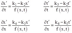
Now, for any choice of the constants A and B, characterizing the slope of the line given by (1), the value of dx/dt must be a constant. This would certainly be the case of the four partial derivatives were themselves constants, meaning that the transformation was purely linear. However, the value of dx/dt would also be constant – for any choice of A and B – if the partial derivatives were of the form

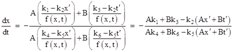
where k₁ to k₆ are constants and f(x,t) is an arbitrary function of f and t. Substituting into the expression for dx/dt, we get

Making use of the fact that Ax′ + Bt′ = −C from equation (1), this reduces identically to the constant

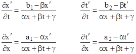
This is consistent with the fact that linear fractional transformations map straight lines to straight lines, as can be seen by examining the partial derivatives of

The partial of this transformation are

Therefore, in the unprimed coordinates, the locus corresponding to (1) has the constant slope

This merely confirms what we already knew, that linear fractional transformations map straight lines to straight lines. To prove that no other functions have this same property, we first need to show that no other functions give partial derivatives of the same form as those of the linear fractional functions. This can be shown by direct integration of the partials back to the original functions.

For completeness, we also need to prove that no other form of partial derivatives yield a constant slope dx/dt for arbitrary values of A and B in equation (2). If the numerator and denominator of the right side of (2) are each constants individually, then any appearances of x and t in those quantities must combine to yield a constant for any values of A and B, given that x and t are transformed from x′ and t′ lying on the locus (1). The only way in which an expression of the form Af(x,t) + Bg(x,t) can be constant for arbitrary values of A and B without the functions f and g being constant is to take advantage of the linear condition Ax′ + Bt′ = −C. This can occur only if the partial derivatives are of the form given above, except that the common denominator can be an arbitrary function of x and t. However, if the denominator is anything other than a linear function of x and t, the integrals of the partials do not lead to satisfactory functions, so these can be ruled out.

The only remaining case to consider is the possibility that the partials satisfy the relations

for some constant K. Then equation (2) would reduce to dx/dt = −K, regardless of the values of A and B. A set of functions that satisfies these conditions is

where k and w are constants. However, these functions imply x′t′ = 1, so these coordinates are not independent, and cannot satisfy equation (1).

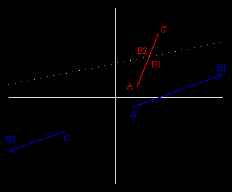
Despite the apparent plausibility of the conditions that enable us to rule out linear fractional transformations, it’s worthwhile to consider whether those conditions are really well founded. Why, for example, must finite coordinates map to finite coordinates?  In general relativity we have the example of Schwarzschild coordinates for a spherically symmetrical gravitational field, and the time coordinate goes to infinity at the Schwarzschild radius, even though the coordinates of the event horizon are finite when expressed in terms of other systems of coordinates. Furthermore, when thinking about the mapping of a particle’s worldline from one system of coordinates to another, we must guard against the tendency to think that the mapping must preserve the causal progression of the particle’s motion. A continuous finite locus of coordinates along a line may map to a discontinuous locus of coordinates along a line, but the discontinuity is in the mapping between the lines, not in the lines themselves. Of course, if we consider only a finite line segment, then a linear fractional transformation may map this to a disjointed line, extending to negative and positive infinity, but with a gap in the middle, as illustrated in the figure below.

Here the red locus is mapped to the blue locus by the transformation

The dotted white line is the locus of points where the denominator of this transformation vanishes. The portion of the red locus from A to B1 is mapped to the semi-infinite line from A to infinity in the direction of B1 on the blue line. The portion of the red line from B2 to C is represented by the semi-infinite blue line extending from infinity in the direction of B2 to C. This admittedly isn’t what we expect intuitively for a transformation from one system of inertial coordinates to another, but it isn’t obvious that such transformations can be ruled out, bearing in mind that we have no a priori right to impose any metrical measure of “distance” on these segments.

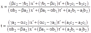
The inverse of transformation (3) is

Letting the origins of the two coordinate systems coincide, we have c₁ = c₂ = 0. Also, we can normalize transformation (3) by setting γ = 1. Now we choose the following values for the coefficients in (3) so that the numerators represent the usual standardized Lorentz transformation:

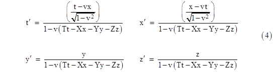
Lastly, we replace the constants α and β with vX and −vT where X and T are constants associated with the transformation. With these substitutions, and adding the y and z coordinates with constants Y and Z for completeness, the original transformation (3) has the form

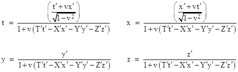
and the inverse of this transformation is

where the accented constants T’, X’, Y’, and Z’ are given by

Thus the inverse transformation is of the same form as the original, except that the sign of v is reversed (as we would expect) and the coefficients T, X, Y, and Z in the denominator are subjected to an ordinary (linear) Lorentz transformation with the parameter v. With v = 0 this reduces to the identity transformation. Of course, if v is not zero, but T = X = Y = Z = 0, we recover the usual linear Lorentz transformation, whereas for any non-zero values of those coefficients we have a linear fractional transformation. It seems conceivable that, for a sufficiently small but non-zero values of the coefficients in the denominator, the difference between the linear fractional and the purely linear Lorentz transformation might be difficult to detect. Notice that small values of those coefficients imply that the plane of inversion (i.e., where the denominator vanishes) is very far away, so finite coordinates would map to finite coordinates for all nearby events. In any case, we have

so null intervals always map to null intervals. In this sense, therefore, the linear fractional transformation (4) evidently possesses the same causal structure as the ordinary linear Lorentz transformations.

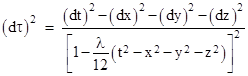
From a physical standpoint, invariance under a linear fractional transformation is not as far-fetched as it might sound, because it is a fact that (for example) Maxwell’s equations are invariant under inversions of the space-time coordinates. Of course, the physical significance of such transformations is questionable, unless some physical meaning could be assigned to the four-vector [T,X,Y,Z] comprising the constant coefficients of the denominator. The transformation involves the “inner product” of this constant four-vector with the coordinate four-vector. Conceivably this vector could be defined on a cosmological basis, such as a four-vector pointing in the time-like direction for a frame of reference in terms of which the distribution of mass-energy in the universe is isotropic. The fact that no such dependence has ever been detected in local physical phenomena obviously implies that the magnitude of such a vector must presently be extremely small in terms of ordinary units – although it need not have always been so insignificant. It would be interesting to know if invariance under this form of linear fractional transformation is consistent with any particular cosmology. In this regard, notice the remarkable similarity between the invariant interval given by (5) and the so-called de Sitter metric, which is a solution of the Einstein field equations and can be written as

where l is the notorious cosmological constant. (See the note Cosmological Coherence for further discussion of this metric.) Of course, this differs from (5) in that no velocity appears in the denominator, and also in that it contains the dot product of the coordinate vector with itself, rather than with the constant four-vector [T,X,Y,Z]. We could eliminate both of these differences and force these expressions into agreement by simply stipulating that the appropriate constants for the denominator of (4) are T = t/v and so on. This still leaves the fact that the numerator in de Sitter’s metric consists of the differentials of the coordinates, whereas the numerator of (5) involves the coordinates themselves, so some re-interpretation is still required to align these two expressions.

Incidentally, during the correspondence between de Sitter and Einstein in 1917, Einstein initially objected to this metric because of the apparent discontinuity that occurs when the denominator vanishes, but de Sitter pointed out that the hyperboloid

intersects the t axis only in the infinite future (and past) when evaluated in terms of natural units. Furthermore, the “singularity” on that hyperboloid is purely a coordinate singularity, not a singularity of the spacetime manifold in terms of the invariant metric.

Return to MathPages Main Menu