From the Field Equations to the Kruskal Metric

Schwarzschild said that half a year was ample time to learn the whole of astronomy. He gave me some books to read and tutored me a little, in exchange for my training him in tennis. When the examination came his first question was: ‘What do you do when you see a falling star?’ Whereupon I answered at once: ‘I make a wish’ – according to an old German superstition that such a wish is always fulfilled. He remained quite serious and continued: ‘Yes, and what do you do then?’ Whereupon I gave the expected answer: ‘I would look at my watch, remember the time, constellation of appearance, direction of motion, range, etc., go home and work out a crude orbit.’ Which led to celestial mechanics and to a satisfactory pass.

                                                            Max Born, 1955

The usual way of arriving at the Kruskal metric for a spherically symmetrical field in general relativity is to first derive the Schwarzschild metric and then make a coordinate transformation that eliminates the singularity in the Schwarzschild time coordinate at r = 2m by “analytically continuing” the geodesics. (This approach is described in another note on radial paths in a spherical gravitational field.) However, the introduction of the singular time coordinate, followed by a transformation that is itself singular at r = 2m, sometimes leaves people uneasy – which is the main reason the actual characteristics of the manifold at r = 2m remained unclear for so many years. The singular behavior of the Schwarzschild time coordinate at and inside the 2m radius can be confusing, and the legitimacy of the transformation procedure can only be established by some fairly sophisticated reasoning. These complications can be avoided (to some extent) by proceeding directly from the Einstein field equations to the Kruskal metric, without introducing the problematic Schwarzschild coordinates.

Our objective is to determine a spherically symmetrical metric that satisfies the vacuum field equations R_μν = 0. Furthermore, to clearly exhibit the causal structure, we would like null paths (which represent the paths of light) to always be at 45 degrees from vertical in a drawing of the coordinates. These conditions immediately imply a diagonal metric of the form

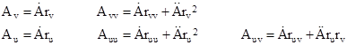
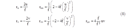
where the parameter r represents the radial position, and A(r) is some function of r, which in turn is a function of the coordinates u and v.  Using dots to denote total derivatives with respect to r, and subscripts to denote partial derivatives with respect to u and v, the partial derivatives of the metric coefficients are

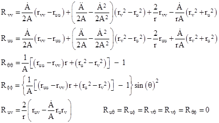
In these terms the components of the Ricci tensor are

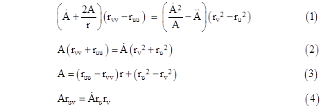
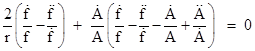
Equating each of these components to zero, we have five conditions, but the condition for R_ϕϕ is redundant to the condition for R_θθ, so we really have just four distinct conditions. It’s convenient to express the conditions imposed by R_vv and R_uu in terms of their sum and difference, so we can express the conditions as

Now, if r is an explicit function of u and v, we could proceed to determine the functions A(r) and r(u,v) from these conditions, but to allow for the possibility that r is an implicit function of u and v, let us consider two functions f and g such that

The partial derivatives of r with respect to u and v are then given by

Equations (2) and (4) give the relation

Substituting for the partial derivatives of r in terms of the functions g and f, and simplifying, we get

This differential equation is satisfied by any arbitrary function of au + bv, and also by any arbitrary function of u² – v². We will find it very convenient later to choose a function h such that huv = 0, which leads to the requirement huu + hvv = 0. The simplest quadratic function satisfying these conditions is simply u² – v². Thus we assure the equivalence of conditions (2) and (4) by setting

which has the partial derivatives

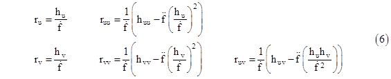
The partial derivatives of r given by (6) can then be written as

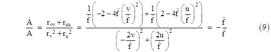
Substituting these expressions into equation (2) gives

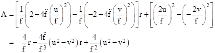
Likewise substituting the expressions (8) into equation (3) gives

Multiplying through by f, and making use of the fact that f(r) = u² – v², this can be written in the form

Differentiating both sides, we get

where

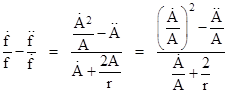
Dividing the left and right sides of this equation by the left and right sides of (10) respectively, the quotient on the left side is

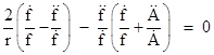
where we’ve made use of relation (9). Subtracting this from the quotient on the right side, we get the differential equation

If we divide through equation (10) by f, and take the derivative of A, and require that the ratio of this derivative to A satisfies (9), we would arrive at this same differential equation for f. Thus if we take a solution of (11) for our f function, and use this compute our A function by equation (10), we will satisfy conditions (2), (3), and (4).

To show that these functions also satisfy condition (1), note that if we substitute from the equations (8) into condition (1) and simplify, we get

Multiplying through by the denominator of the right hand side, this gives

Again making use of (9), this can be written as

This would be equivalent to (11) if

which is automatically satisfied given that (9) is satisfied, as can be seen by taking the derivative of the relation

Differentiating this expression gives

Dividing through by the derivatives of A and f, we get

which is the same as (12). Therefore, with h(u,v) given by (7), and with f(r) being a function that satisfies (11), and with A(r) computed from (10), all of the components of the Ricci tensor vanish, so we have a solution of the vacuum field equations.

To characterize the solutions of (11) in a systematic way, we can express f(r) as a Laurent series expansion, but after substituting this into (11) we find that all the coefficients of negative powers of r must be zero, which implies that f(r) must be analytic, i.e., it must have a power series representation of the form

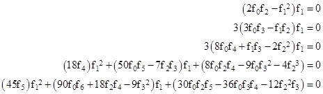
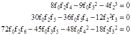
Substituting this into (11) and setting the coefficients of each power of r to zero, we have the following conditions on the coefficients.

and so on. If f₁ is not zero, then the first condition shows that f₀ and f₂ must also be non-zero. In this case we can freely choose arbitrary (non-zero) values f₀ = α and f₁ = β, and the remaining coefficients are then fully determined, having the values

and so on. Therefore, in this case (i.e., with f₁ ≠ 0) the function f(r) is of the form

for arbitrary constants α and σ = β/a. The corresponding function A(r), given by equation (10), is

Recalling that the value of r in this expression is a function of u and v given by the relation f(r) = u² – v², we can write r and A explicitly as functions of u and v.

Thus we have the line element

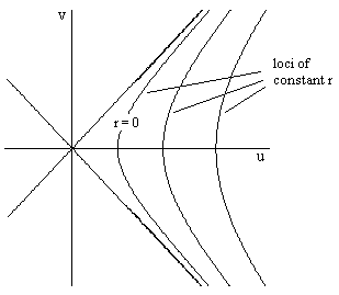
For this system of coordinates the radial position r = 0 corresponds to the hyperbolic locus of points with u² – v² = α, and all positive values of r are in the right-hand quadrant as shown in the figure below.

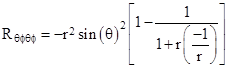
Notice that a light ray from the point r = 0 and v = 0 can propagate freely to all larger values of r, which might seem contrary to our expectation for a gravitational field. But notice also that no source mass appears in this metric. It is simply a non-inertial coordinate system for flat Minkowski spacetime. To confirm this, we can evaluate the components of the full Riemann curvature tensor, and show that they are all zero for this metric. It’s particularly useful to evaluate the component R_θϕθϕ in terms of r, θ and ϕ, because these three parameters have the same physical significance for all of our metrics as well as for the Schwarzschild metric, permitting a direct comparison. For the general family of metrics described above, it can be shown that

Inserting the function f(r) = αe^σr and the corresponding expression for A(r) into this equation, we find R_θϕθϕ = 0, whereas for the Schwarzschild metric we have

Thus the above metric corresponds to the case m = 0. From this we conclude that no line element of the desired form can represent a gravitational field with m ≠ 0 if the coefficient f₁ in the power series expression for f(r) is non-zero. Therefore we return to the conditions for the coefficients of the power series, but this time we set f₁ = 0. The result is that the first three conditions are automatically satisfied, without imposing any restriction on the values of f₀, f₂, and f₃. The remaining conditions are

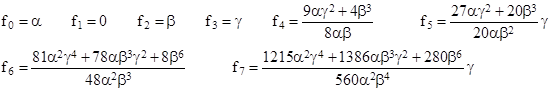
and so on. In this case we can freely choose f₀ = α, f₂ = β, and f₃ = γ, and then recursively compute all the remaining coefficients from these conditions. This give the coefficients

and so on. Notice that the odd coefficients are all multiples of γ, so if γ = 0 the function f(r) is an even function of r. In that case the non-zero coefficients are

and so on. Therefore, in this case we have

where σ = β/α. Since A(r) is zero, the metric is singular for the u and v coordinates. Moreover the reference curvature component, given by (13), is

which is infinite for any non-zero value or r. If we take r = 0 the metric vanishes completely, so this “Gaussian” expression for f(r) doesn’t lead to a realistic field.

Therefore we require f₃ ≠ 0. In a sense, the three non-zero parameters f₀, f₂, and f₃ represent three degrees of freedom for the solutions of (11), setting aside the flat solution and the singular “Gaussian” solution. For any specified values of these three coefficients, equation (11) uniquely determines all the remaining coefficients. The only solutions in finite polynomials are of the form

for arbitrary values of a, σ, and n. Furthermore, these constitute all the solutions of (11) (aside from the flat and Gaussian), because the series expansion of this function is

so for any given values of f₀, f₂, and f₃ we can compute

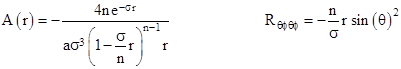
Since (11) gives unique values for all the remaining coefficients, and since (16) represented solutions with all possible values of these initial coefficients, it follows that all the solutions of (11) (aside from the flat and Gaussian) are of the form (16). The corresponding metric coefficients and reference curvature are

For any value of n other than 1, the metric coefficient A either vanishes or becomes infinite at r = n/σ. Therefore, to give well-behaved metric coefficients for all positive values of r, we must set n = 1, and for convenience we also set a = –1, leading to the functions

Thus we have the line element

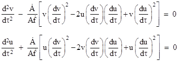
which is finite and non-singular at every positive radial location. We can already see that the value of σ must be 1/(2m) in order for the curvature component R_θϕθϕ to equal the corresponding component given by (14) for the Schwarzschild metric for a gravitational field of mass m. However, this would be making essential use of the Schwarzschild solution, because the value of R_θϕθϕ for Newtonian gravity is zero. To complete the derivation without invoking the Schwarzschild solution at all, we need to determine the value of σ more directly. This amounts to determining the value of the gravitational constant, which we’ve taken as unity by choosing suitable units. In practice this is based on empirical observations of the inverse square relation for the radial acceleration of gravity from rest. To evaluate this relation in terms of σ, we must first determine the geodesic equations for the metric. We only need to consider the radial and time components, because we will work with fixed angular values of θ and ϕ. Evaluating the Christoffel symbols and inserting them into the expressions for the geodesic equations for the two-dimensional space with coordinates u and v, we get

We note in passing that for null geodesic paths (i.e., light pulses) we have dv/dτ = ±du/dτ, in which cases these equations reduce to

and therefore such paths continue in the “45 degree” direction with dv/dτ = ±du/dτ.

Now, we wish to determine the acceleration experience by a test particle at rest at a radial position r from a mass m, assigning to r and m the approximate physical meanings they have in Newtonian gravity, and evaluating the acceleration in terms of the proper time of the particle. Thus we wish to find d²r/dτ² based on the metric (17) for a test particle that is at rest (meaning dr/dτ = 0) on the u axis at the radial position r corresponding to some initial u₀. Differentiating the relation

we have

which shows that the condition dr/dτ = 0 at v = 0 and u = u₀ requires du/dτ = 0. From this and the metric (17) it follows that, at the initial condition, we have

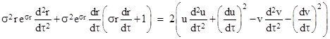
Furthermore, differentiating (19) again, we get

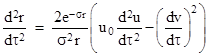
Inserting the values for our condition and solving for d²r/dτ², this reduces to

We can get the second derivative of u from the second geodesic equation for this condition

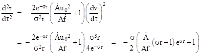
Substituting this into the previous equation, we get

where we’ve made use of (18) and (20) for our specified conditions. Inserting the functions A and f, this reduces to

It follows that we must have σ = 1/(2m) in order to match the Newtonian inverse-square relation d²r/dτ² = –m/r². Therefore the line element (17) must be

where r is given as a function of u and v implicitly by the relation

This completes the derivation of the Kruskal metric directly from the field equations, without transforming from, or making any use of, the Schwarzschild coordinates.

Return to MathPages Main Menu