The Cayley-Hamilton Theorem

Every square matrix satisfies its own characteristic equation. This interesting and important proposition was first explicitly stated by Arthur Cayley in 1858, although in lieu of a general proof he merely said that he had verified it for 3x3 matrices, and on that basis he was confident that it was true in general. Five years earlier, William Rowan Hamilton had shown (in his “Lectures on Quaternions”) that a rotation transformation in three-dimensional space satisfies its own characteristic equation. Evidently neither Cayley nor Hamilton ever published a proof of the general theorem. References to this proposition in the literature are about evenly divided in calling it the Cayley-Hamilton theorem or the Hamilton-Cayley theory. The first general proof was published in 1878 by Georg Frobenius, and numerous others have appeared since then.

Depending on how much of elementary linear algebra and differential equations we take for granted, the proof of the Cayley-Hamilton theorem can be fairly immediate. For an arbitrary square matrix M with characteristic equation f(z) = 0, the general solution of the linear system  is given by x(t) = e^Mtx(0). We also know that each component of x(t) individually satisfies the differential operator form of the characteristic equation, so we have f(d/dt)x(t) = 0. Inserting the expression for x(t), we get f(M)e^Mtx(0) = 0, and since this must be true for any initial conditions x(0), it follows that f(M) = 0, which was to be proven.

However, this proof could be criticized for taking too much for granted. It makes use of the exponential form of the general linear system solution, and of the fact that x satisfies the differential operator form of the characteristic equation. These are familiar and not very difficult propositions, but it might be argued that they are no more self-evident than the fact we are trying to prove.

As an alternative, consider again the homogeneous linear first-order system , where x is a column vector, M is a constant square matrix, and dots signify derivatives with respect to t. The general solution can be expressed in the form x = Cε where C is a constant square matrix and ε is a column vector given in terms of the eigenvalues λ₁, λ₂, …, λ_n, not necessarily distinct, by

where the a_j exponents are zero for the first appearance of a given eigenvalue and incremented for each subsequent appearance. The derivative of x is , so we can substitute for x and x’ in the original system equation to give. Multiplying through by the inverse of C, we get . Hence if the eigenvalues are all distinct, the matrix C^–1MC is simply the diagonal matrix of the system’s eigenvalues, and we immediately have f(C^–1MC) = 0. Furthermore, noting that C(C^–1MC)ⁿC^–1 = Mⁿ, it follows that C f(M) C^–1 = 0 and so f(M) = 0.

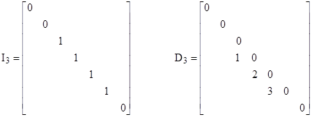
If there are repeated eigenvalues, then C^–1MC is the sum of the diagonal matrix of the system’s eigenvalues plus a “differentiation matrix”. For each distinct eigenvalue λ_j with multiplicity m_j, let I_j denote the diagonal matrix with unit elements in each location where λ_j occurs, and let D_j denote the differentiation matrix comprised of integers counting the repeated eigenvalues, placed to the left of the diagonal locations of the respective eigenvalues. For example, if a seventh-order system has eigenvalues λ₁, λ₂, λ₃, λ₃, λ₃, λ₃, λ₄,  then the I₃ and D₃ matrices are

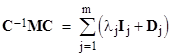
In terms of these matrices, we have

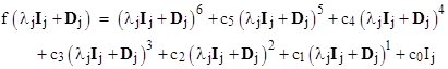
where m is the number of distinct eigenvalues. The matrices for the distinct eigenvalues are independent, so it suffices to show that f(λ_jI_j + D_j) = 0 for arbitrary j in order to prove that f(C^–1MC) = 0. To show this, we can substitute directly into the polynomial as follows:

Letting k denote the number of copies of the eigenvalue in this component, we can expand the powers and re-arrange terms to give the expression

The matrix D_j^k is identically zero, and each of the other terms also vanish because λ_j is a root of the first k–1 derivatives of f. Therefore, we’ve shown that f(C^–1MC) = 0, even when there are duplicated eigenvalues. By the same argument as before, it then follows that f(M) = 0, completing the proof.

Incidentally, these two proofs of the Cayley-Hamilton theorem mirror the Heisenberg and Schrödinger versions of quantum mechanics. Both proofs begin with the linear system , but they proceed on the basis of two different explicit solutions, i.e., the solutions x(t) = e^Mtx(0) and x(t) = Cε(t). In the first case the solution is given as a time-dependent operator applied to a constant vector (as in Heisenberg’s matrix mechanics), whereas in the second case the solution is given as a constant operator applied to a time-dependent vector (as in Schrödinger’s wave mechanics).

Return to MathPages Main Menu