On the Origins of Quantum Mechanics

An incompatibility between the concepts of position and motion was already apparent to philosophers in ancient times. For example, around 500 BC Zeno of Elea asked what was physically different, at any given instant, between an arrow in motion and an arrow at rest. Since nothing moves in an instant, he argued that the motion of an object cannot be manifest in any given instant, from which it follows that, although an arrow has a precise and definite position at any given instant, its state of motion is completely indeterminate (if it can be said to exist at all in that instant). Conversely, to determine the motion of an arrow, the arrow must be observed over some interval of time, but in that case its position becomes indeterminate, because its position changes during any interval of time. Thus, even from this primitive perspective, one can see that position and motion (i.e., the rate of change of position with time) are incompatible attributes in the sense that their pure manifestations exist only on mutually exclusive bases. Position is manifest in an instant but motion is not. Motion is manifest over an interval of time, but position is not. From this we might wonder if both attributes can be exhibited exactly in a single elementary interaction.

Of course, if we regard position, time, and motion as continuous and infinitely divisible, we can formally resolve the incompatibility by evaluating both position and motion over an interval of time in the limit as that interval goes to zero. However, Zeno also pointed out various problematic aspects of the idea of a continuous world with infinitely divisible attributes, and one can argue that the inconsistency of this idea is apparent even in very commonplace phenomena. For example, it’s intuitively clear that the energy of a physical system tends to distribute itself uniformly over all available energy modes. However, a continuous system possesses infinitely many energy modes, extending to infinitely great frequencies, so the energy of any stable physical system ought to be almost entirely in the infinitely high frequency modes – which is why this conundrum is called the ultra-violet catastrophe.

To illustrate, consider a solid bar of steel, struck with a hammer at its midpoint. The energy conveyed to the bar will initially be mostly in the lowest frequency vibrational mode of the bar, but with the passage of time the energy will disperse into higher harmonics. This dispersal of energy to higher frequencies (and lower amplitudes) continues until reaching the quantum scale, i.e., the scale on which the seemingly continuous metal bar is actually seen to consist of discrete irreducible entities (atoms), at which point the energy approaches thermodynamic equilibrium. Thus the energy of the original hammer strike has been dispersed into agitation of the discrete particles, corresponding to an increase in the temperature of the bar. We can show that the total energy has been conserved, provided we account for mechanical energy and thermal heat energy once the bar has reach its limiting state. However, this thermodynamic equilibrium is possible only because the steel bar is not continuous, but actually consists of discrete irreducible entities. If the bar were truly continuous, the energy would continue forever migrating toward higher and higher frequencies (and smaller and smaller amplitudes), never reaching equilibrium at any finite scale, so the energy would soon be in a form that could never appreciably interact with entities on the scale of the original disturbance. In effect, there could be no thermodynamics, and no conservation of energy, because mechanical energy would effectively vanish into the realm of infinitely high frequencies (and infinitesimal amplitudes).

Considerations of this kind might have suggested the earliest “quantum” theory, namely, the theory of atomism, first proposed by a few philosophers in ancient Greece, and later revived by Gassendi, Dalton, and others. The development of this original quantum theory – which posited that matter exists only in discrete packets of finite mass – proceeded hand-in-hand with the development of the kinetic theory of matter. Underlying this theory was the notion of the vacuum, i.e., empty space, within which the discrete individual particles of matter were thought to exist and move. We might call the vacuum a plenum of possibilities, as opposed to the plenum of actualities (i.e., substance) in the tradition of Aristotle and Descartes. These two competing ideas have continued to be relevant and viable even to the present day.

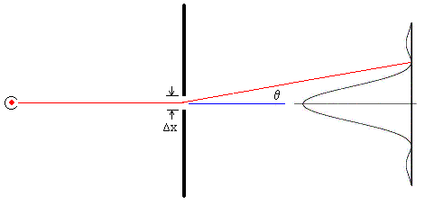
From the preceding discussion we’re led to expect that position and momentum (which is the appropriate quantification of “motion”) will be found to be mutually incompatible when examined on the irreducible scale that necessarily exists in order to make possible the existence of thermodynamic equilibrium. We don’t have to look far for evidence of this incompatibility, because it is clearly exhibited by the ordinary diffraction of light, a phenomenon first noted by Francesco Grimaldi around 1640. (His findings were published in 1665). The figure below shows a source of monochromatic light (the red dot on the left) shining through an aperture of width Δx and then onto a screen. The curve on the right indicates the intensity of the light striking each point.

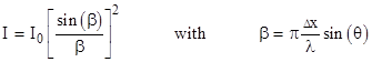
For a sufficiently small aperture and sufficiently distant light source and screen, the intensity of the light emerging from the aperture at an angle θ is

where λ is the wavelength of the light. The first minimum occurs at β = π, and if we insert this value into the definition of β, we see that it corresponds to an angle θ satisfying the equation

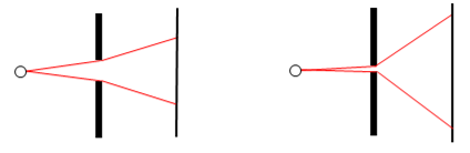
Thus the characteristic range of diffraction angles for light rays passing through an aperture is inversely proportional to the size of the aperture. A wide aperture yields small diffraction angles, whereas a narrow aperture yields wide diffraction angles, as illustrated schematically in the figures below.

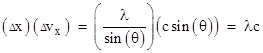
We also know that each pulse of light is moving with the speed c, so the rays moving at an angle θ will have a speed in the x (vertical) direction of sin(θ) times c, which implies that the velocity (in the x direction) of a pulse in passing through the aperture of width Δx changes by the amount

This is a measure of the uncertainty of the velocity in the x direction for light that has passed through the aperture. Hence we have the relation

showing that, for a given wavelength (i.e., for a given frequency) of light, the product of the uncertainty in position and the uncertainty in velocity is a constant, and this constant is proportional to the wavelength. Thus, in a very immediate and tangible way, the ordinary diffraction of light exemplifies the incompatibility between position and motion. By reducing the size of the aperture we more precisely fix the position in the x direction of the pulse of light, but this broadens the intensity distribution of the light pulse, so that it’s motion in the x direction becomes more indeterminate.

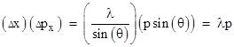
Furthermore, letting p denote the momentum of a pulse of light, the change in momentum in the x direction is Δp_x = p sin(θ), so we have

We presume the total momentum p of an elementary pulse of light is constant (since its speed is constant), but in addition we can appeal to the previous discussion (involving the ultra-violet catastrophe) to assert that motion is not infinitely divisible, and hence that there must be a fundamental unit of momentum for electromagnetic radiation of a given wavelength. Let this quantum of momentum be given by p = h/λ, where h is a constant (Planck’s constant). Substituting this into the above equation gives the Heisenberg uncertainty relation

This discussion was based on the diffraction of light, but matter waves corresponding to massive particles exhibit diffraction of exactly the same kind, so the Heisenberg uncertainty relation is universal.

This is such an important result that it’s worth trying to get a clear understanding of why it’s true. The phase associated with the amplitude for a photon to travel from the light source through the aperture and on to a certain point on the screen depends on the total path length, which varies depending on where the path crosses the aperture. If the aperture is wide, there will be a wider range of phases combining at a given reception point on the screen. This results in more complete cancellation for points away from the central axis. Conversely, if the aperture is very narrow, the only available paths from source to screen are all of nearly the same length, so there is very little cancellation, even for points far from the axis. This is essentially identical to the incompatibility described by Zeno, because the motion (in the x direction) of a particle only manifests itself over a non-zero range of possible positions in the aperture, whereas the position manifests itself precisely only for an aperture of zero width.

In view of this fundamental incompatibility between the position and momentum of elementary entities, we conclude that the classical way of conceiving of physical systems is inapplicable – at least on the scale of elementary discrete actions. Recall that the usual way of representing a physical system in the classical context is in terms of a set of configuration (position) coordinates, and the “trajectories” of those coordinates, i.e., the derivatives of the configuration coordinates with respect to time. To assign the appropriate weights to different coordinates, we also specify masses, and multiply the configuration derivatives by their respective masses to give momenta. Thus for a system with n degrees of freedom we have n configuration coordinates and n momentum coordinates. Each configuration coordinate has a corresponding momentum. Given a full and precise specification of both the configuration and the momentum of a system, classical laws of dynamics typically allow the computation of the second time derivatives of the configuration coordinates, which can then be used to extrapolate the momentum into the future (or past), and likewise the momentum can be used to extrapolate the configuration. However, as we’ve seen, the two components of the information necessary to specify (classically) the physical state of a system – namely the position and the momentum coordinates – are mutually incompatible. At the level of elementary entities, we might say (paraphrasing Mikowski’s famous remark about space and time) that position by itself, and momentum by itself, are doomed to fade away into mere shadows, and only a kind of union of the two will preserve an independent reality.

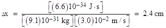
The uncertainty principle leads immediately to an apparent paradox. If an object of mass m is known to be moving (in the x direction) at the speed v (assumed small compared with c) with an uncertainty of Δv, it follows that the precision Δx to which the object’s position x can be known is

For example, if the velocity of an electron (in the x direction) is known with an uncertainty of ±3 cm/sec, the minimum possible uncertainty in the electron’s position is on the order of

These are appreciable uncertainties, so one might wonder why we don’t observe such limitations when dealing with macroscopic objects. Now, a superficial answer would be to point out that for objects with larger masses the product of the velocity and position uncertainties is less. If we replace the electron in the preceding example with a hydrogen atom, consisting of a proton and an electron bound together, we find that the uncertainty in the position is just 13 microns, which is re-assuringly small. However, since the electron is part of this atom, and shares its motion, haven’t we succeeded in determining both the position and the velocity of the electron to a precision that violates the uncertainty relation? We can raise the same question about the constituent parts of any object, i.e., the uncertainty relation implies that – for a given uncertainty in the velocity – the uncertainty in the positions of the individual constituent parts must be greater than the uncertainty in the position of the aggregate of all the parts. This is impossible, so we can only conclude that in any bound aggregate of parts there must be more uncertainty in the velocities of the parts than in the velocity of the bound aggregate. For example, when we specify that the velocity of a hydrogen atom has an uncertainty of ±3 cm/sec, we are referring to the center of mass of the atom, and the electron is in motion relative to that center. Hence the uncertainty in the velocity of the electron is much greater than that of the overall atom.

One might think this could be used to evade the uncertainty principle, simply by having a particle follow a “zigzag” path, such that there is a large uncertainty in the microscopic velocity (on each individual zig and zag), while there is a much smaller uncertainty in the net velocity (averaged over many zigs and zags). Indeed this possible, but of course it requires the particle to be “anchored” to another mass, and so it leads again to an aggregate of bound parts, with the uncertainty in the aggregate’s position and velocity being inversely proportional to the total mass. Thus the classical limit of sharply defined positions and velocities for macroscopic objects is possible only because the elementary constituent parts of such objects are in relative motion, and their individual velocities are highly uncertain, even though their combined average velocity is well-behaved. This corresponds to the fact that, assuming independence, the deviations of the means are related to the deviations of the individual elementary particles by

Thus we have

The requirement for independence necessitates relative motions between the constituent particles of an aggregate body. This lack of coherence is crucial, because if the particles were somehow to all be in a coherent state, the resulting body would exhibit appreciable quantum effects, on the macroscopic scale. The chaotic motions associated with the temperature of an ordinary macroscopic body normally ensures independence between the velocities of the elementary constituent particles, but we might surmise that bodies whose temperatures are reduced to near zero might, in some circumstances, exhibit quantum effects on the macroscopic scale.

Another inference that can be drawn from these relations is that, for tightly bound aggregates of particles, for which the positional variations of the individual particles are limited, the (independent) velocity variations must increase. Hence we could deduce something like Boyle’s law for macroscopic substances. Of course, carried to the extreme, this also enables us to account for the stability of (for example) the hydrogen atom, because as the electron’s position is bound more and more closely to the proton, the variation of its velocity must increase, so we eventually arrive at an equilibrium condition.

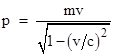
Still another consequence of these relations can be seen if we remove our assumption that all the velocities are small compared with the speed of light. We know empirically that no matter or energy propagates faster than light, which seems to place an upper limit on the variation (uncertainty) in the velocity of a particle. This, in turn, would imply a lower limit on the uncertainty in the position of a particle. And yet we do not observe any such limit on positions, i.e., we seem to be able to make a particle exhibit a position with arbitrarily great precision. The resolution of this conflict comes, of course, from the fact that the uncertainty relation actually depends on momentum rather than velocity, and the momentum p of a particle of (rest) mass m and speed v is not really mv but rather

Thus variations of velocity in the finite range from –c to +c correspond to variations in momentum in the unbounded range from –∞ to +∞. This allows a particle to exhibit (in principle) specific and definite values of either position or momentum.

The diffraction of light (or matter) waves through an aperture, as discussed above, is just one example of how, when a physical entity interacts with its surroundings in such a way as to exhibit its spatial position precisely, the momentum of the entity becomes indeterminate. Likewise when an interaction exhibits the momentum precisely, the spatial position becomes indeterminate. According to one of the usual formalisms of quantum mechanics, the state of a physical system is represented by a state vector, whose temporal evolution is governed by a certain linear equation as long as the system remains isolated from its surroundings. (This is somewhat problematic, because all physical systems interact gravitationally with each other at all times, so it’s unclear whether there even exist any truly isolated systems. For purposes of ordinary quantum mechanics, any effects of gravitational interactions are normally neglected.) Interactions with the surroundings are represented by various operators, each of which corresponds to a classical observable variable, such as position or momentum.

By means of an interaction, the system exerts an effect on its surroundings, and the surroundings exert an effect on the system. One might expect the formalism to be explicitly symmetrical, since the surroundings can also be regarded as a system, but in its customary form quantum mechanics is not symmetrical in this sense. The effect of the system on the surroundings is represented by the appearance of one of the operator’s eigenvalues. Hence this information (i.e., the result of the “observation” or “measurement” of the corresponding variable) is emitted from the system into the surroundings. But in the other direction, the interaction has the effect of modifying the system’s state vector so that it becomes the eigenvector corresponding to the exhibited eigenvalue. Thus in one direction the effect is represented as merely the introduction of one of the operator’s eigenvalues for the “observed” variable, whereas in the other direction the effect is represented as a transformation of the system’s state vector into one of the eigenvectors of the operator.

The particular eigenvalue that emerges as a result of any given “observation” is apparently selected at random (a somewhat vaguely criterion) from the operator’s set of eigenvalues. This fundamental indeterminacy was among the features of quantum mechanics to which Einstein objected. Interestingly, one of his favorite ideas for an alternative explanation of quantum phenomona was a kind of over-determination.

We might try to imagine a more symmetrical formulation of quantum mechanics, in which (for example) a measurement of the momentum of a system can just as well be regarded as a measurement of the “inverse momentum” of the surroundings. One of the obstacles to this approach is the fact that the operators, or equivalently the matrices, representing observable variables don’t act algebraically. If we apply the measurement represented by the matrix M to a system with the state vector V, the resulting state vector after the measurement is not given by MV. Rather, it is given by a vector U such that MU = λU for some eigenvalue λ of M. Given that the choice of eigenvalue is probabilistic, there is no direct algebraic way of arriving at U from V and M. There are iterative algorithms for finding an eigenvalue, but they typically determine only the dominant eigenvalue. To represent quantum phenomena we would need an algorithm that returns each eigenvalue (and the corresponding eigenvector) with a probability proportional to the squared norm of the respective diagonal coefficient. It isn’t easy to imagine an algorithm – at least in the usual sense of the word – that would yield just one of a set of possible results when applied to a given state vector, and such that the choice of results would satisfy all reasonable tests of randomness.

To give just one example of a deterministic mathematical structure that exhibits what could be regarded as probabilistic effects – and to illustrate the inadequacy of such a structure for representing quantum mechanical processes – recall that any given polynomial of degree d with integer coefficients can be associated with a sub-group of the symmetric group S_d, and this determines the “probabilities” (in sense described below) that the polynomial will factor over the integers modulo a randomly chosen prime p in each of the possible ways. For example, a polynomial of degree 5 considered modulo a certain prime p may be irreducible, or it may factor into polynomials of degree 4 and 1, or into polynomials of degree 3 and 2, and so on. In all, we have the following seven possible types of factorizations of a quintic polynomial:

If the group of a given quintic polynomial is the fully symmetric group S₅, each of these seven types of factorizations is possible. Moreover, to each of these factorization types we can assign a weight proportional to the number of permutations possessing the corresponding cyclic decomposition. Thus the factorizations of type {5} have the weight 24, because there are 24 permutations of 5 elements with a single cycle. The weights of the seven factorization types respectively are

Now, as Cheboterov proved, the asymptotic fraction of primes p such that the polynomial factors into one of the possible factorization types is proportional to the respective weight. The distribution of the primes into these seven categories seems to be completely random, governed only by the requirement that the asymptotic densities correspond to the weights listed above. In other words, the splitting field of the polynomial modulo an arbitrarily chosen prime can be any one of the seven possible types, with probability proportional to the weight of that type. Hence we could draw an analogy between the possible factorization types of a polynomial and the eigenvalues of a measurement operator. The weight of a particular factorization type would correspond to the probability of a particular eigenvalue. Of course, the “observation” of a given polynomial modulo a given prime always yields the same result, so each act of observation must be associated with a different prime, which then requires us to stipulate how this association is to be established. The possible mappings are so arbitrary that the analogy is not very satisfactory.

Return to MathPages Main Menu