Markov Models with Aging Components

The original defining property of Markov models was that the state transitions were memoryless, which is to say, the transition times are all exponentially distributed with constant rate parameters. The time variable enters into the governing equations only in the differential sense, insofar as the derivatives of the state probabilities with respect to time appear. The equations are independent of the absolute value of time, so any arbitrary value can be taken as the time origin. For this reason, such models are said to be homogeneous in time. Moreover a single time parameter suffices for the coordination of the entire model, so such models possesses temporal coherence.

More general models, in which the transition rate parameters are allowed to vary as functions of the time, are said to be non-homogeneous in time (viz, they behave differently depending on the absolute value of the time). However, such models may still be based on a single coherent time parameter, so they are still not suitable for modeling the behavior of systems for which the state transitions vary as functions of the ages of the components. In a system with aging components, renewals of those components will generally result in a range of multiple distinct ages for the components of the system in any given state. Such a system could be regarded as homogeneous in time, because the behavior does not depend on the absolute value of time, but it does depend on the ages of the components relative to their renewal times. Of course, the “age” of each component can be regarded as a time variable, so the model is not time-homogeneous in that sense, but more significantly, no single time variable suffices to coordinate such a system, because each component must carry its own age – and in fact must carry a distribution of possible ages – as the overall system evolves. Therefore, even though the system is still (in the sense indicated) homogeneous in time, it does not possess temporal coherence.

As an aside, the concept of multiple time parameters, one for each component (particle) of a system, has been discussed in the context of quantum mechanics. Recall that, in non-relativistic quantum mechanics each coordinate of the position (and momentum) of each particle must be treated as a separate dimension, and the laws governing the behavior of the system operate within this higher-dimensional “phase space”. In a sense, the spatial coordinates of the various components are allowed to be decoherent, but a single coherent time parameter is retained. It has often been suggested that, to do justice to a relativistic version of quantum mechanics, in which the time and space coordinates play comparable roles, we ought to allow each entity to have its own time dimension, so the phase space of n entities would have 4n instead of just 3n positional dimensions. Although this is a very compelling idea, no one has ever succeeded in developing it into a full theory. Roger Penrose commented that “a basic difficulty with allowing each particle its own separate time parameter is that then each particle seems to go off on its merry way off into a separate time dimension”.

This same “basic difficulty” is encountered in Markov models used in reliability analysis, when the failure rates of the components are allowed to be functions of the ages of those components, so each one effectively has its own time coordinate. However, aside from Monte Carlo simulations, the usual approach is to treat these systems as inhomogeneous yet coherent in time, i.e., to assume that a single time parameter suffices to coordinate the system evolution. As a result, it can be applied only to system in which each component “goes off on its merry way”, with no interaction between them. In other words, the model must be “factorable” into the individual component histories, each of which can be separately evaluated, so the combined model is really just a formal aggregation of independently evolving components. To treat analytically the general renewal problem for systems with rates that depend on the ages of the components, the most important feature is not inhomogeneity, but rather decoherence.

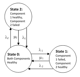
To illustrate, consider a simple system consisting of two redundant components, each of which may be in one of two states, healthy or failed, and suppose we allow for repairs of failed components at constant rates. If the failure rates of the components are constant, and if we stipulate that both components are repaired immediately if they are both failed, then the Markov model for the system is as shown below.

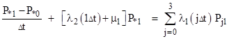
The failures of the second components are shown returning to the fully renewed state, because the fully failed state is repaired immediately. The two state equations for this homogeneous model are

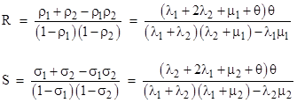
along with the gauge condition P₀ + P₁ + P₂ = 1. This system of equations is easily solved for the transient behavior for any given initial condition. Also, by setting the derivatives to zero, we can solve for the steady-state probabilities

where

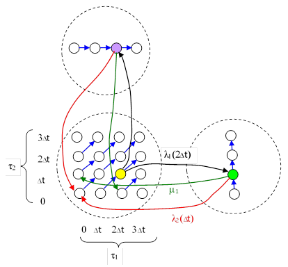
Now suppose that instead of constant failure rate parameters λ₁ and λ₂, each of the components has a failure rate parameter that is a function of the age of that component since it was last renewed. We will let τ₁ and τ₂ denote these ages. For clarity, we will begin with discrete functions, and let the failure rate parameters be specified for four discrete ages, 0, Δt, 2Δt, and 3Δt. For each macro-state with n healthy components we must account for 4ⁿ micro-states, representing all possible combinations of ages for the n operational components. (The age of a failed component is irrelevant.) Hence the complete Markov model representing this system is as shown below.

The blue arrows in this figure represent the aging transitions, each with a rate parameter of 1/Δt. Only a few of the failure and repair transitions are shown, but all the others follow the same pattern of the ones shown. The shaded yellow micro-state represents the fully functional state in which the ages of the two operational components are τ₁ = 2Δt and τ₂ = Δt respectively. Therefore, the failure transition to the macro-state with the first component failed has a rate parameter of λ₁(2Δt), and since the age of the second component doesn’t change at the instant of failure of the first, this transition flows into the micro-state (shaded green in this drawing) with τ₂ = Δt. There are only two ways of exiting the green micro-state (in addition to the aging transition). First, there could be a failure of the second component, in which case the system is totally renewed, so it flows back to the full-up state with ages  τ₁ = τ₂ = 0, as shown by the red path. Second, the first component could be repaired, which would renew the first components but would not affect the age of the second. Hence this transition would flow into the full-up state with  τ₁ = 0, τ₂ = Δt, as shown by the green path. The transitions from the yellow full-up state to the upper macro-state, and back, are defined similarly.

This system consists of 24 micro-states in all. We can evaluate the time-dependent response of such a model by treating it as a Cauchy problem. In other words, we specify the density functions of all the states at some initial time, and then we have equations giving the rates of change of those density functions as a function of time. However, in the remainder of this note we will focus on determining the steady-state solution of such a model. It should be noted, however, that the time required for decoherent model to reach steady-state may be very great, so in practical applications (such as reliability analysis) consideration should be given to the time-dependent solution.

To solve for the steady-state probabilities and flow rates, we set the derivative of each state probability to zero, so the flow into each state equals the flow out of that state. This gives us 24 linear equations in the 24 unknown micro-state probabilities which, together with the gauge equation (sum of all probabilities is unity) can readily be solved. It’s convenient to designate the micro-states by subscripts denoting the ages (in increments of Δt) of the operational components, with asterisks (*) for the ages of the failed components. With this notation, the steady-state equation for the yellow micro-state in the above diagram is

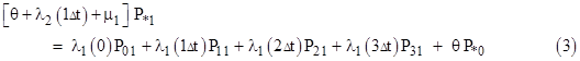
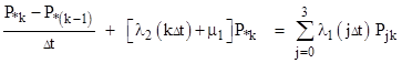
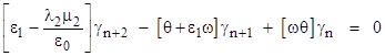
where θ is the aging rate parameter, i.e., θ = 1/Δt. There are nine equations of this type. The steady-state equation for the green micro-state, taking into account that it is fed by all the full-up micro-states with τ₂ = Δt, is

There are eight equations of this type, except that the boundary states lack one of the “θ” aging transitions. The equation for the micro-state immediately below the yellow micro-state is similar to that for the yellow micro-state, except that it receives flow from the purple state in the drawing above, and it receives no “aging input”, because it is in the zeroth row. Thus we have

There are six equations of this type. Finally, the equation for the single completely renewed full-up state is

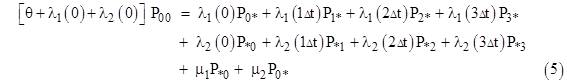
The gauge condition for this model is

This can be used in place of the equation for the fully-renewed state.

Notice that equation (3) for the green micro-state can be expressed in the form

More generally, for any of the microstates in the macrostate with the first component failed, we have

for any k greater than zero. (Boundary states are exceptions, because they lack one or the other of the aging transitions, but those will be treated appropriately when we sum these microstates to determine the probabilities of the macrostates.)

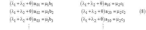
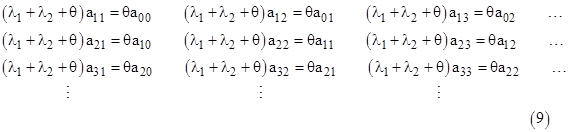
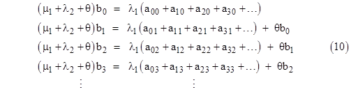
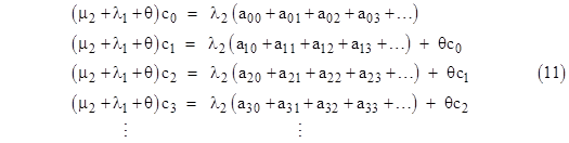
Even with constant failure rates, this approach can be used to determine the steady-state distributions of ages within each of the states of the model. Let’s consider the same model again, but this time with constant rates λ₁, λ₂ and a larger number of time increments. Letting a_ij , b_j, and c_j denote the probabilities of macrostates 0, 1, and 2 respectively, the steady-state system equations are

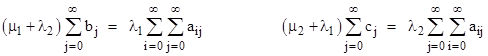
To check the validity of these equations, first notice that the sum of equations (10) and the sum of equations (11) give, respectively, the relations

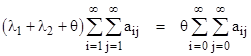
which are just the steady-state system equations (μ₁ + λ₂)P₁ = λ₁P₀ and (μ₂ + λ₁)P₂ = λ₂P₀.  Also, summing all of equations (7) and (8) together, we get

Now, the sum of equations (8) is

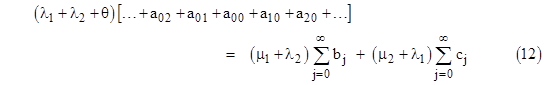
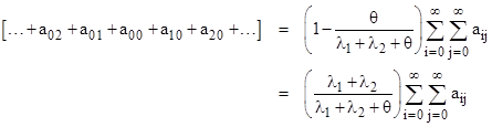
and from this it follows that the sum of the “perimeter” probabilities is

Substituting this into (12) gives

which is just the sum of the basic system equations.

Before algebraically solve these equations, it will be useful to solve the discrete system numerically by integrating the time-dependent equations to give the age distributions for a system with constant failure rate parameters of λ₁ = (50)10^-6 per hour and λ₂ = (20)10^-6 per hour, and repair rate parameters of μ₁ = 1/100 and μ₂ = 2/1000. The age increments are approximately 10000 hours so, for example, the probability of the system being in the full-up state with the age of the first component in the range 20000-30000 hours, and the age of the second component in the range 40000-50000 hours, is 0.00594.

State 0:

       0      1      2      3      4      5      6      7      8      9     10

 0  .08711 .04025 .03355 .02796 .02330 .01941 .01618 .01348 .01123 .00936 .00780

 1  .02563 .05124 .02368 .01973 .01644 .01370 .01142 .00952 .00793 .00661 .00551

 2  .01717 .01508 .03014 .01393 .01161 .00967 .00806 .00672 .00560 .00467 .00389

 3  .01145 .01010 .00887 .01773 .00819 .00683 .00569 .00474 .00395 .00329 .00274

 4  .00763 .00673 .00594 .00522 .01043 .00482 .00402 .00335 .00279 .00232 .00194

 5  .00509 .00449 .00396 .00349 .00307 .00614 .00283 .00236 .00197 .00164 .00137

 6  .00339 .00299 .00264 .00233 .00206 .00181 .00361 .00167 .00139 .00116 .00097

 7  .00226 .00200 .00176 .00155 .00137 .00121 .00106 .00212 .00098 .00082 .00068

 8  .00151 .00133 .00117 .00104 .00091 .00081 .00071 .00062 .00125 .00058 .00048

 9  .00100 .00089 .00078 .00069 .00061 .00054 .00047 .00042 .00037 .00073 .00034

10  .00067 .00059 .00052 .00046 .00041 .00036 .00032 .00028 .00025 .00022 .00043

State 1:

       0      1      2      3      4      5      6      7      8      9     10

    .00081 .00068 .00057 .00048 .00040 .00033 .00028 .00023 .00019 .00016 .00013

State 2:

       0      1      2      3      4      5      6      7      8      9     10

    .00306 .00218 .00146 .00097 .00065 .00043 .00029 .00019 .00013 .00009 .00006

Note that this solution was based on a finite model extending only out to 400000 hours, and we have printed only out to the first 100000 hours. Such systems can always be solved numerically, either by integrating the dynamic equations until they reach steady state, or by explicitly solving the steady-state system equations. It appears that the age distributions have an exponential form, as predicted, but we can also see that the boundary microstates are discontinuous from the rest of the states. We also see that the effect of this discontinuity appears to propagate along the diagonal of State 0, although the non-diagonal microstates seem to conform (at least roughly) to the expected joint exponential distribution.

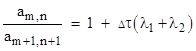
Notice that along each diagonal the ratio of successive terms is very closely equal to 1.70. This can be understood from the basic governing equations (9), which give

This is exact for the discrete case. In the following we will let ω denote the reciprocal of this ratio, i.e., we define the parameter

To explicitly solve the entire set of equations (7)-(11) we first observe that the sum of the equations is zero, so they are not independent. Also, the equations are homogeneous, so we can omit (7), and divide all the other variables by a₀₀ to give the new set of normalized variables

We can solve the system equations (absent (7)) for these variables, and then determine the absolute values of a₀₀ and the original variables by invoking the gauge equation, i.e., the requirement that the sum of all the probabilities is unity.

For convenience we define the following parameters to denote certain frequently occurring quantities:

Now begin by using equations (8) and (10) to determine a recurrence relation for the values of β_n. We can write the third of equations (10) as

Making use of the ratio ω, the quantity in parentheses on the right side can be written as

The sum on the right side of this equation appears in the second of equations (10), so we can make that replacement to give

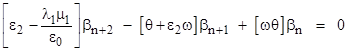
Now we can substitute for α₀₂ from equation (8), re-arrange terms, and generalize the indices on the values of β_n, (noting that the same relation applies to all), to give the second-order homogeneous recurrence

This is valid for all n = 0, 1, 2, …   The characteristic roots of this recurrence are

Likewise the sequence of γ_n values satisfies the recurrence

and the characteristic roots of this recurrence are

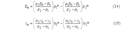
In terms of these roots, the values of β_n and γ_n can be written explicitly as

Hence, given β₀, β₁, γ₀, and γ₁, we can compute all the β_n and γ_n values, from which we can compute the values of α_0n and α_n0 using equations (8), and finally all the remaining α_mn values using equations (9). It only remains to determine the four values β₀, β₁, γ₀, and γ₁.

We haven’t yet made use of the first members of the equation sets (10) and (11), so we can use them (after normalization) to impose conditions on the four principal unknowns. Substituting for the α_mn values in the first normalized equations of sets (10) and (11), we have

The sums of the β_n and γ_n values can be expressed in terms of geometric series using the preceding formulas. For example, the sum of all the β_n values is

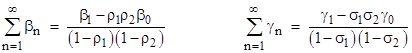
and similarly for the γ_n values. From this we get the following expressions for sums beginning from the index n = 1:

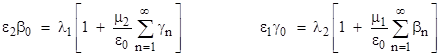
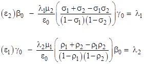
Inserting these sums into the previous equations, we get two equations in the four principal unknowns:

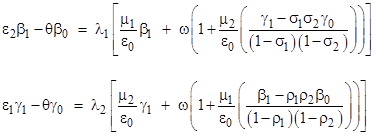
Repeating this for the second members of the normalized sets (10) and (11), and making use of (8) to eliminate the extra α values, gives two more equations in the four unknowns

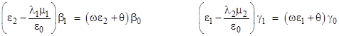
These two equations can be simplified by using the previous two equations to eliminate the expressions for the summations. When this is done, the equations reduce to

Recalling the coefficients of the characteristic polynomials, we see that these equations can be written as

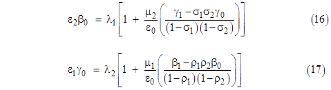
Making these substitutions into (16) and (17), we get two equations in the two unknowns

Solving these equations gives the result

where

For the numerical example whose solution was tabulated above, these formulas give

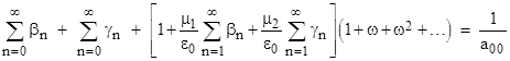
With these values, equations (14) and (15) can now be used to compute all of the β_n and γ_n values, and then equations (8) and (9) give all the α_mn values, noting that α₀₀ = 1. It only remains to determine the absolute value of a₀₀, which we do by imposing the gauge condition, i.e., setting the sum of all the probabilities to 1. This implies that the sum of all the normalized variables is 1/a₀₀. We sum all the variables as follows

Evaluating these summations, we get

Inserting the numerical values from our tabulated example, we get the value a₀₀ = 0.08711…, in agreement with the table. Also, multiplying the β_n, γ_n, and α_mn values by a₀₀ gives values of b_n, c_n, and a_mn in agreement with the table.

The results of this note are extended to cover continuous models (i.e., in the limit as Δt goes to zero) in the article entitled Age Distributions in Continuous Markov Models.

Return to MathPages Main Menu