Waves in Ascending and Descending Dimensions

There are some remarkable relationships between elementary spherically symmetrical solutions of the wave equation in spaces of different dimensions. As discussed in the note on spherical waves in higher dimensions, by the separation of variables we can split the wave equation into spatial and temporal parts, and the spatial part f(r) satisfies the differential equation

where n is the number of spatial dimensions. (We’ve chosen units such that the wave length equals unity.) Letting f_n denote a solution of (1) in a space of n dimensions (and one time dimension), the function given by

is a solution of (1) in space of n+2 dimensions. To prove this, note that the definition of g(r) implies (after multiplying through by –n/r and differentiating)

where dots signify derivatives with respect to r. Also, differentiating equation (1) gives

Substituting for the derivatives of f_n from the preceeding expressions, we get

Simplifying this expression, we get

which proves that g(r) is a solution in space of n+2 dimensions. Thus we have a sequence of solutions in ascending dimensions

Interestingly, this can also be expressed as a sequence of (scaled) solutions in descending dimensions. To see this, use equation (1) to replace the left side of (2), and then multiply through by –r/n to give

Integrating both sides, we get (up to a constant of integration)

Now we multiply through by r^n–1 to give

The expression inside the square brackets is simply the derivative of rⁿf_n+2, so this can be written as

Thus if we define the scaled wave function F_n(r) = r^n–2 f_n(r), we have

In other words, F_n is simply a scaled derivative of F_n+2, so this gives a sequence of solutions in descending space dimensions, by a formula very similar to equation (2).

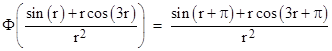
At this point we should note that the negative sign in (2) is potentially misleading, because the negation can be accomplished either by multiplying by negative 1 or by applying a phase shift to the periodic parts of the function, specifically by subtracting π from the phase. As discussed in the note on fractional calculus, a generalized differentiation operator applied to the sine or cosine function amounts to a simple phase shift, and this just happens to give negation when the phase shift is π. Therefore, instead of writing equation (2) with a leading factor of –1, we will write it with a leading factor of Φ^–1, where Φ is a linear phase shift operator defined by

where g is a periodic function. Linearity means that Φ(a+b) = Φ(a) + Φ(b). For example,

Using this operator, we will take as the general form of equation (2) the expression

We can make use of either (3) or (5) to derive simple explicit expressions for elementary wave solutions in n dimensions, for both odd and even values of n. First, notice that in view of the identity

we can express equations (3) and (5) in the form

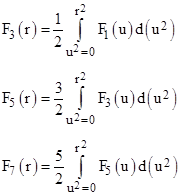
Given the elementary one-dimensional solution F₁(r), the left hand relation allow us to determine a sequence of solutions by repeated integration as follows

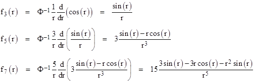
and so on. Now, in one-dimensional space we have the elementary solution f₁(r) = cos(r), which in scaled form is F₁(r) = cos(r)/r. Therefore we have

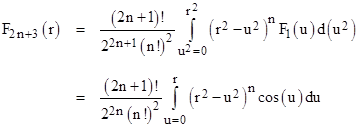
and hence f₃(r) = sin(r)/r as expected. Integrating again (with the appropriate scale factor) on F₃ gives F₅, and so on. Thus, using Cauchy’s formula for repeated integration (see the note on fractional calculus for a derivation of this useful formula), we can express F_2n+3 by performing the integration n+1 times. The product of the leading scale factors is

so the repeated integrations give the formula

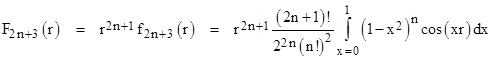
Factoring an r²ⁿ out of the integrand and making the substitution x = u/r, this can be re-written as

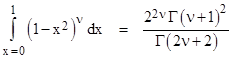
As discussed in the note on fractional calculus, the natural generalization of this (n+1)th order integral is to allow n to be a non-integer ν, and replacing the factorial of n with the gamma function of ν+1. Thus we arrive at

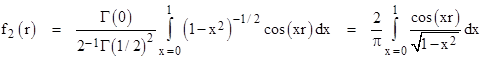
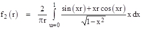
For space of two dimensions we set ν = –1/2 in the above formula to give the solution

This agrees with the result found in the note on Huygens’ Principle by means of a series evaluation, and we note that it is the lowest-order Bessel function, i.e., f₂(r) = J₀(r).

Incidentally, with regard to equation (6), it’s worth noting the identity

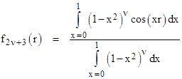
Thus equation (6) can be written in the form

which shows that the wave function is the mean of cos(xr) on the interval from x = 0 to 1 with the density proportional to (1–x²)^ν. 

An alternative approach to developing wave solutions in n dimensions is to use the ascending sequence of solutions given by equation (5), beginning with the elementary one-dimensional solution f₁(r) = cos(r), as follows

and so on. Thus the ascent from n dimensions to n+2 dimensions is given by applying the differential operator

Applying this operator n times to a one-dimensional solution gives an expression for a 2n+1 dimensional solution. So, on this basis, our expression for higher-dimensional solutions is

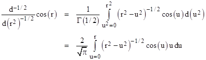
Since each differentiation (with respect to r²) raises the number of space dimensions by two, we need to apply a half-order differentiation to produce solutions for spaces with even numbers of dimensions. Using the Left Hand Rule for fractional differentiation, we first perform a half-integration on sin(r) with respect to r² by means of Cauchy’s formula, which gives

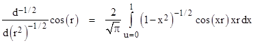
Dividing out the r², and making the substitution x = u/r, and noting that du = r dx, this can be written as

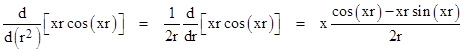
We now need to perform one whole differentiation with respect to r², and we can do this inside the integration. Noting that

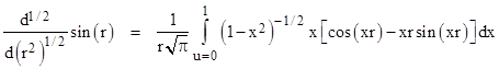
we finally arrive at the half-derivative of cos(r)

Inserting this into equation (7) with n = 1/2 gives

This again equals the Bessel function J₀(r), although the equivalence is non-trivial. Thus we can arrive at consistent results using the sequence of solutions related by differentiation in either the ascending or descending space dimensions.

The correspondences between solutions in higher and lower dimensions is essentially one-to-one, and all the solutions in higher dimensions can be mapped down to (or up from) a solution in one dimension. Using the series solution technique described in the note on Huygens’ Principle, it can be shown that all one-dimensional solutions are of the form

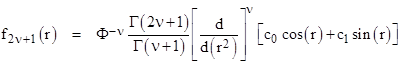
for some constants c₀ and c₁. So, returning to equation (7), generalizing to non-integer orders by replacing n with the real value ν and replacing the factorials with gamma functions, and inserting the general one-dimensional solution in place of the special solutions cos(r), we have

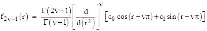
The phase shift and differentiation operators are commutative, so we can apply the shift to the basic argument, and write this in the form

This shows that for any given number of space dimensions there is a two-parameter family of solutions. Also, for any choice of those two parameters we can vary the number of dimensions continuously.

Return to MathPages Main Menu