Markov Models with Boolean Transition Logic

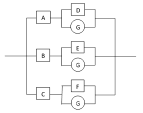
A wide variety of systems can be accurately represented as complete Markov models with Boolean transition logic. In general, a system consisting of N bi-state components can be represented by a Markov model with 2^N states with specified transition rates between the states. As discussed in the note on Complete Markov Models, these transitions can be encoded as Boolean logic, which greatly facilitates the modeling task. In addition, the steady-state solution can be computed very efficiently by a simple numerical approach, similar to solving potential flow fields with specified boundary conditions by iteratively applying the local steady-state conditions. As an example, consider the system shown schematically in the figure below.

Each of the three main operational paths represents a separate replaceable unit, and each of them has components (denoted by A, B, C) whose failures are detectable, and another set of components (D, E, F), whose failures are undetectable, and whose function is to provide protection against a common external threat (G), such as a lightning strike. Each of the components has has a specified random failure rate, and the external threat has a certain random rate of occurrence (which may or may not be specified). In addition, if the external event G occurs while D is failed, then component A fails, and likewise for the other two units. The repair strategy is based entirely on the states of the detectable components A, B, C. If any one of them is failed, the system is allowed to operate for a fixed amount of time, T₁ hours, and then the affected unit is repaired. Whenever a unit is repaired, its external threat protection function is checked and (if found to be failed) repaired. If any two of the detectable components is failed, the system is only allowed to complete the current mission, for a mean time of T₂ hours, and then the affected units are repaired. The failure of all three units represents complete system failure. Our objective is to determine the mean system failure rate.

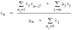
This model contains four main types of transitions: (1) simple random failures of the individual components, (2) repairs triggered by the failures of the respective components, (3) repairs triggered by failures of other components, and (4) failures triggered by a other component failures and/or external events. The general formula for the steady-state content ratio of each state, taking into account all of these types of transitions, was given in a previous note as

The only non-trivial aspect of this expression is the second summation in the numerator, which requires knowledge of every state j that has a “repair” flow into state n. To evaluate this summation efficiently, it is worthwhile to pre-determine, for each state in the model, the state into which it flows when “repaired”. The word “repaired” is placed in quotes, because in our more general model we can specify transitions from less-failed to more-failed states.

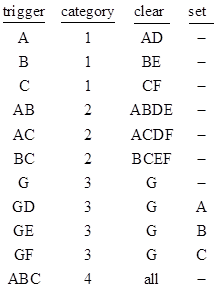
In general, a system model can be defined by specifying a set of “triggering” mincuts, and for each trigger specifying (1) a transition category with an associated rate, (2) a set of components to be failed (i.e., cleared), and (3) a set of components to be repaired (i.e., set). For example, the model described above can be represented by the following information

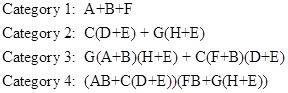
Given this information, the category of each state can be determined as the highest category for any triggering mincut contained in that state. Once the category of a given state is known, we can then determine the state into which the given state flows by ANDing the state’s binary index with the complement of each “clear” mincut in that category, and ORing with each “set” mincut in that category. The result is the binary index of the state into which the given state flows. The rate of this flow is specified by the category of the given state. For this example, the value of μ for each category 1 state is 1/T₁, and for each category 2 state is 1/T₂. The values of μ for the category 3 is set to some large value, to give an essentially instantaneous rate, because the external threat (e.g., a lightning strike) is treated as a momentary event. If the protection features are healthy, the lightning strike comes and goes with no effect, whereas if the protection features are failed the lightning strike state immediately flows into the affected unit failure state. Hence essentially no time is spent in any of the lightning strike states. They serve merely to trigger the transitions to other states. Lastly, the values of μ for the category 4 states are set to some large value, although is really arbitrary, since the value drops out of the final system failure rate.

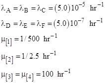
Thus to complete the model definition, along with the above table, we must specify the m values for each category, and we must also specify the random failure (or occurrence) rate for each component (or event). To give a concrete example, we can take

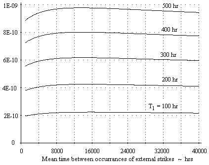
The only remaining information needed to evaluate the system failure rate is the value of λ_G, which is the rate of occurrence of the external threat. Often this rate is not known, especially because it represents the rate of occurrences severe enough to damage a unit if the protection features have failed. One useful approach is to evaluate the system failure rate for a range of external threat rates, and choose the most conservative value. (This strategy is described in more detail in the notes Redundant Systems With a Common Threat and Undetected Failures of Threat Protection.) Given the complete model definition, we can solve for the steady-state system failure rate by iterating on the system state equations. A BASIC implementation of this algorithm is shown in the appendix. The figure below shows the failure rate of this system as a function of λ_G for T₁ values ranging from 100 to 500 hours.

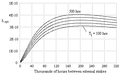
This shows that the system failure rate is relatively insensitive to the rate of occurrence of the external threat. However, this is not always the case. For example, if the detectable failure rates for the three units were each reduced by a factor of five, the system failure rate as a function of the external strike rate for various values of T₁ would be as shown below.

To show the versatility of this modeling technique, note that the identical program can be used to represent the sample system described in Complete Markov Models by specifying the following information.

This represents 22 triggering mincuts, and minimal repair strategy is given by clearing each component in any mincut that satisfies the condition of the event category. In this example there are no “set” components. Assigning suitable values of λ_A through λ_H, and for μ_[1] through μ_[4], we get the system discussed in the referenced note.

As an aside, it’s interesting that the program shown in the attachment is somewhat analogous to a universal Turing machine. The “data” provided to this program consists of an arbitrary set of Boolean expressions on N variables, along with two classes of transition rates, one intrinsic to each variable, regulating the “local” transitions, and another representing the effects of certain Boolean combinations. In effect, the program “simulates” any defined sequence of logical operations on the N variables by controlling the “flow” of probability through the network of 2^N states. If these features are applied to the time-dependent version of the program (discussed a previous note), the resulting routine has the capability of simulating the operations of a very large class of programs. Of course, all systems expressible in this form are linear (assuming all the transition rates are finite), so their long-term behavior can, in principle, be determined in a finite number of steps by explicitly constructing and solving the full 2^N x 2^N transition matrix. One way of expanding the computational range still further would be to allow the number N to be infinite, with Boolean transition rules applicable to infinite sets of states. The program might resolve the system consisting of just one component, then two, then three, and so on, until satisfying some halting criterion. Another approach would be to allow the controlling Boolean rules to be modified by the state probabilities. Still another generalization would be to allow for non-linear transition laws, e.g., replacing the flow λP with a flow of the form λP(1−P).

Return to MathPages Main Menu