Rotation Matrices

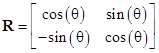
In two dimensions the general rotation can be expressed in terms of Cartesian coordinates by a matrix of the form

for any constants a and b. There is only one degree of freedom, and we can normalize by setting a² + b² = 1. Thus there is a constant θ such that a = cos(θ/2) and b = sin(θ/2), and so the transformation can be written in the familiar form

Since the determinant of a rotation is unity, equation (1) relies on the Pythagorean sum-of-squares formula

Thus any rotation based on integer values of a and b corresponds to a Pythagorean triple. In fact, it corresponds to a 2 x 2 orthogonal orthomagic square of squares. (The term orthogonal means the row vectors are mutually perpendicular, as are the column vectors, and the term orthomagic means that each row and each column of the squared elements sums to the same constant.) In general, the component R_ij of a rotation matrix equals the cosine of the angle between the ith axis of the original coordinate system and the jth axis of the rotated coordinate system. In other words, the elements of a rotation matrix represent the projections of the rotated coordinates onto the original axes. Naturally this relation is reciprocal, so the inverse of a rotation matrix is simply its transpose, i.e., R^-1 = R^T. The eigenvalues of (1) are

with the corresponding eigenvectors

Of course, any complex multiples of these eigenvectors are also eigenvectors. Notice that we can present two multiples of each eigenvector as the rows and columns respectively of a 2 x 2 matrix as shown below

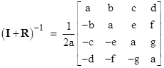
Letting R denote an arbitrary (two-dimensional) rotation matrix as in (1), and letting I denote the identity matrix

it’s easy to show that

We also have the interesting identity

Noting that the determinant |I + R| equals the scalar quantity 4a² / (a² + b²), the above can also be written in the form

We also note that the determinant of (I – R) is 2(1–cos(θ)), which is non-zero for any θ other than a multiple of 2π, so except in those cases we can multiply on the right by the inverse (I – R)^–1 to give the expression

This is a (scaled) similarity transformation, so any two-dimensional rotation matrix R is similar to (I + R)² in this sense. In fact, since R commutes with I – R, we have

for two-dimensional rotations. We’ll see below that closely analogous (but not identical) formulas apply to rotation matrices in three and even (in a restricted way) four dimensions as well.

Extrapolating the form of equation (2), we consider a 3 x 3 matrix R such that

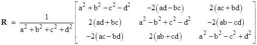
for arbitrary constants a,b,c,d. Solving this for R gives

There are only three degrees of freedom in this rotation, so we can normalize by setting a² + b² + c² + d² equal to unity. The determinant of the matrix inside the brackets (without the leading factor) is simply the sum a² + b² + c² + d², and since determinants are multiplicative, it isn’t surprising that the determinant of the product of two such matrices is given in terms of the determinants of the original matrices by the “sum-of-four-squares” formula. This is analogous to Fibonacci formula for the product of two sums of two squares. The real eigenvalue of the transformation is λ₁ = 1, and the corresponding eigenvector has components proportional to (b,c,d), so this vector points along the axis of rotation. The only remaining parameter is a (divided by the square root of the determinant, which we have normalized to 1), which must therefore represent the amount of rotation about that axis. Just as in the two-dimensional case, we find that a = cos(θ/2) for a rotation through the angle θ. It follows that b² + c² + d² = sin(θ/2)², again assuming normalized values for a,b,c,d.

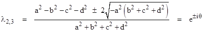
The three dimensional rotation matrix also has two complex eigenvalues, given by

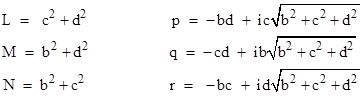
In terms of the parameters

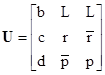
the eigenvector corresponding to λ₂ is proportional to each of the columns of the matrix

and the eigenvector corresponding to λ₃ is proportional to each of the rows. The barred variables are complex conjugates. The columns of this matrix are mutually orthogonal, as are the rows (so to this extent the matrix has the properties of a rotation). The sum of the squares of the components of each vector (row and column) is zero, whereas the sums of the squared norms of the components of the rows (and of the columns) are 2LD, 2MD, and 2ND respectively, where D = (b² + c² + d²). The determinant of this matrix is zero, and the eigenvalues are 0, 0, 2D. The eigenvalues of the symmetrical part are 0, D, D, and the eigenvalues of the anti-symmetrical part are 0, –D, D.

Any three non-parallel eigenvectors comprise a basis. Taking one representative from each of the three eigenvectors as the columns, we can form the matrix

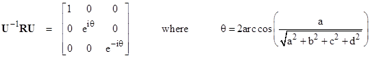
Then by the usual similarity transformation we can diagonalize the rotation matrix as follows

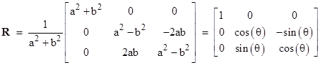
It’s interesting to consider the physical significance of the complex eigenvectors for rotations in three dimensions. Since the set of rotation matrices is closed under multiplication, it follows that any re-orientation in space can be expressed as a pure rotation about some fixed axis. If we choose our coordinate system so that the axis of rotation coincides with one of the coordinates axes, then the rotation matrix degenerates to essentially a two-dimensional rotation. For example, for a rotation about the x axis we have c = d = 0, and the three-dimensional rotation matrix reduces to

In this case the real eigenvector is just (b,0,0) and the two complex eigenvectors are represented by the rows and columns (respectively) of the matrix

which of course represents just the two complex eigenvectors from the two-dimensional case.

Incidentally, this rotation can also be expressed in terms of quaternions. In general, letting v’ denote the vector given by applying to the vector v a rotation through an angle θ about the axis defined by the vector (b,c,d). The quaternion operation for determining v’ is by means of the formula

This is an elegant formulation, but the multiplications involved in the quaternion products actually require more elementary operations than the matrix multiplication.

The analog of equation (3) is

We also have the determinant

which shows that the analog of equation (4) for three-dimensional rotations is

However, for three-dimensional rotations, the determinant of I – R is identically zero, so in this case we cannot multiply through by the inverse (as we did in the two-dimensional case) to give an analog of equation (4’). We also note that (6) differs from equation (4) by the factor of 2 on the right hand side.

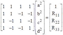
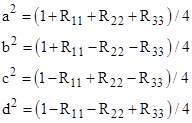
Given the diagonal elements of R, we can compute the normalized parameters by means of the relations

Solving these equations gives

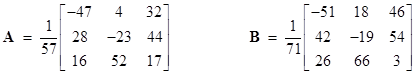
We could define a rational rotation as one for which the values of a, b, c, and d are rational. These can be generated by taking integer values of the parameters, without normalizing them. For example, setting the parameters to 1,2,4,6 or to 1,3,5,6 gives the two rational rotation matrices

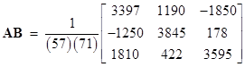
Incidentally, squaring each of the elements in each bracketed matrix gives a 3 x 3 orthomagic square of squares. The product of these two matrices is another rational rotation

corresponding to the parameters –61, –1, 15, 10, which are related to the parameters of the A and B matrices by the sum-of-four-squares formula.

It’s tempting to extrapolate from equations (2) and (5) to higher dimensions. This would lead us next to define a 4 x 4 matrix R by the relation

for constants a, b, c, d, e, f, g. By analogy with the previous cases, we might hope the determinant of this matrix would be the sum of the squares of the seven parameters divided by 16a², but this is the case only if we impose the condition

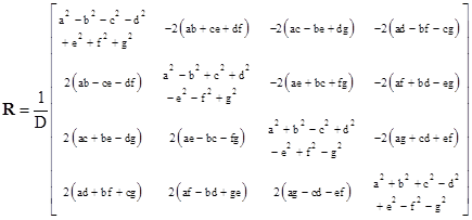
With this condition, we can indeed carry through the derivation of the four-dimensional rotation matrix

where

This matrix satisfies all the usual requirements of a rotation matrix, such as the fact that the rows are mutually orthogonal, as are the columns, and the sum of the squares of each row and of each column is unity. The seven parameters are constrained by two conditions (the normalizing condition and the special condition bg – cf + de = 0), so there are five degrees of freedom (which is less than the six degrees of freedom for the fully general rotation in four dimensions because of the extra constraint we have imposed). Analogous to equations (4) and (6), we have

which is identical to the earlier equations except for the coefficient 4. It appears that the coefficient for N-dimensional rotations (restricted as necessary) equals 2^N–2. As in the three-dimensional case, the determinant of I – R in the four-dimensional case is identically zero, so again we cannot multiply through by the inverse to get an analog of (4’). For more on this topic, including the fully general four-dimensional rotation matrix with six degrees of freedom, see the note on Rotations and Anti-Symmetric Tensors.

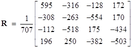
As an example of a four-dimensional rotation matrix, let the parameters a through g have the values 1, 2, 4, 6, 9, 20, and 13 respectively. Notice that we have put f = (bg + de)/c so these parameters satisfy the requirement bg – cf + de = 0. The resulting four-dimensional rotation matrix is

The squares of the elements inside the brackets constitute a 4 x 4 orthomagic square of squares, with the common sum equal to the square 499849 = 707².

Return to MathPages Main Menu