Periodic and Continuous Repair Models

Consider a triply-redundant system consisting of three identical components, each with a constant failure rate λ, checked and repaired periodically once every τ hours. Between inspections, the system continues to function as long as at least one of the three components is working. If the system totally fails, it is repaired (or replaced) immediately. We will consider two methods of determining the long-term system failure rate. First, the exact solution will be computed as the mean rate given by the time-dependent solution over a time period of τ hours, beginning from the fully-operational state. Second, we will show how this exact result can be very closely approximated by a simple steady-state model with suitably chosen repair rates.

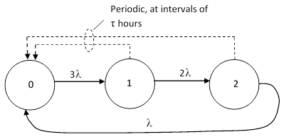
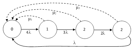
The system can be represented by the Markov model (with periodic repairs) shown below.

Between periodic transfers the time-dependent system equations are

from which we get the eigenvalues of the system

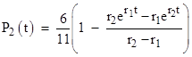
in terms of which the time-dependent probability of state 2 is given by

for constants A, B, and C. If we take P₀(0) = 1 we have the initial conditions

(The initial value of the second derivative is easily determined by the method described in the note on Feynman’s Ants.) This implies the solution

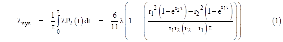
The system failure rate as a function of time is λP₂(t), and we can evaluate the mean failure rate for one period from t = 0 to τ by integrating this rate and dividing by τ as follows

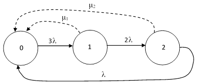
The second approach is to approximate the periodic repairs as continuous transitions with constant rates, as shown in the figure below.

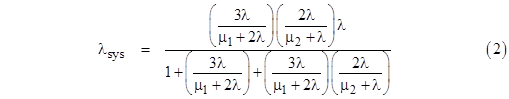
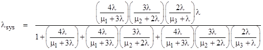
The overall system failure rate is λP₂, and the steady-state system can be solved algebraically to give

To approximate the effect of the periodic repairs, we will choose values of μ₁ and μ₂ that give the same mean time to repair for systems entering states 1 and 2 respectively during an interval of length τ. One simple approach is to conservatively set all the rates equal to 1/τ, which is roughly equivalent to use an exposure time of τ hours for each component in a fault tree model. On the other hand, a less conservative approach is given by subtracting from τ the mean time for a system to arrive during the interval for a simple open-loop model. For a system with N redundant components, it can be shown that the mean time to repair for the k-fault state, neglecting any intermediate repairs, is given by

For example, given a system with just N = 2 components, the continuous repair rate corresponding to a periodic inspection and repair interval of τ hours from the single-fault state could be approximated by

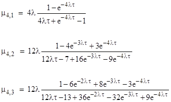
Likewise for a system with N = 3 components (as in the previous examples), the continuous rates for the states with one and two faults can be approximated by

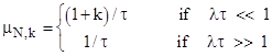
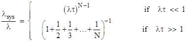
It’s easy to show that these rates are asymptotic to

These are extremely close approximations in their respective regimes, so we only need to be concerned about choosing a suitable rate when λτ is on the order of unity. We can conveniently encompass both the asymptotes and interpolate smoothly between them by simply using the rates

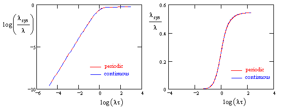
Using these values for the repair rates μ₁ and μ₂ in equation (2), we can compare the overall system failure rate based on the continuous repair model with the rate given by equation (1) for periodic inspection and repairs. The result is shown in the plot below.

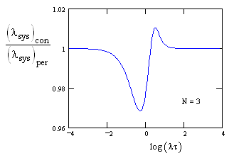
We see that the results are virtually indistinguishable, and this is confirmed by the plot of the ratio between the two methods shown below.

To investigate this further, consider a system with N = 4 components, as represented by the model shown in the figure below.

In this case the continuous repair rates given by equation (3) for the states with one, two, and three faults are

But, again, it is preferable to use to rate given by equation (4) as

The steady-state solution for the continuous model is

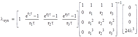
The corresponding system failure rate with strictly periodic repairs can be expressed in the form

In order to compute the system failure rate in this case we need to determine the three non-zero eigenvalues r₁, r₂, and r₃, which are the non-zero roots of the characteristic polynomial

Thus we have

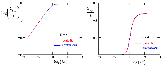
Making use of these values, we can plot the continuous and periodic solutions for the case N = 4 as shown below.

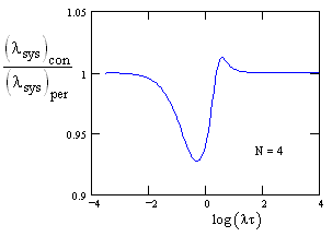
This again shows that the results are nearly indistinguishable, as confirmed by a plot of the ratio of the two calculations shown below.

The asymptotes for large and small lt are identical, and for lt near zero the most extreme ratio is about 0.93, representing a difference of about 7%.

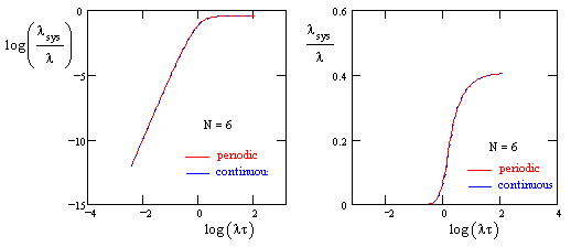
Carrying this a couple of steps further, the plot below shows the exact periodic solution for N = 6 along with the corresponding continuous solution.

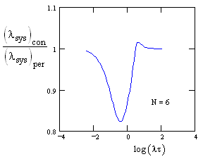
Even in this case, where the total system failure involves the joint failure of six independent components, the strictly periodic solution and the corresponding continuous solution give nearly indistinguishable results. A plot of the ratio of these two solutions is shown below,

As always, the deviation from 1 is appreciable only for lt near unity. In this case, the most extreme ratio is about 0.82, representing a difference of about 18%.

In general, for N identical components, the continuous solution can be written in the form

where

Inserting the asymptotic values of μ into this equation gives the two asymptotic failure rates

Return to MathPages Main Menu